Table of Contents
Composite walls are often used in Industrial equipment’s and building structures to get the desired heat transfer. The overall heat transfer coefficient is widely used in thermal engineering to evaluate the heat transfer rate across complex systems such as composite walls, heat exchangers, and other multi-layered structures.
The overall heat transfer coefficient (U) is a measure of the total resistance to heat transfer through a composite system, that includes all modes of heat transfer (conduction, convection, and radiation).
Overall Heat Transfer Coefficient is defined as the amount of heat transferred per unit area per unit temperature difference between the two sides of a composite wall or system.
Related: Inverse Square Law for Radiation
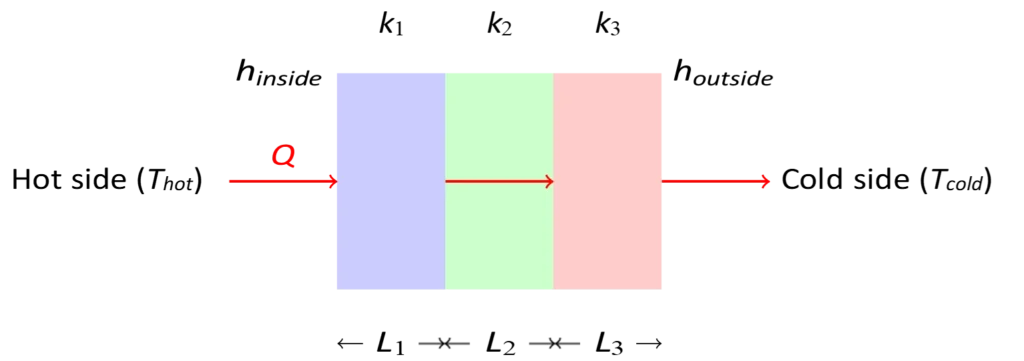
For the given fig. 1 the overall heat transfer coefficient can be calculated using the formula given below:
\[U = \frac{1}{\frac{1}{h_{\text{i}}} + \frac{L_1}{k_1} + \frac{L_2}{k_2} + \frac{L_3}{k_3} + \frac{1}{h_{\text{o}}}}\]
where:
- \( h_{\text{i}} \) is the convective heat transfer coefficient on the inside.
- \( h_{\text{o}} \) is the convective heat transfer coefficient on the outside.
- \( L_1, L_2, L_3 \) are the thicknesses of the three layers.
- \( k_1, k_2, k_3 \) are the thermal conductivities of the three layers.
Related: Heat Transfer through Convection Calculator – Newton’s Law of Cooling
Overall Heat Transfer Coefficient Calculator
This calculator helps used to calculate the Overall Heat Transfer Coefficient (U) and the Heat Transfer Rate (Q) for a system with multiple layers of materials. User will be able to input the thickness and thermal conductivity of each layer, convective heat transfer coefficients on the inner and outer sides, and the temperatures on both sides.
Note: For single-layer heat conduction, set the thicknesses of the other layers to zero. This will remove those layers from the calculation, leaving only the single layer of interest.
Related: Kirchoff’s Law of Thermal Radiation, Wien’s Displacement Law
Related: Joule-Thomson Effect – Coefficient Calculation for CO2 and N2
Thermal Resistance through composite walls
Thermal resistance is a measure of a material’s ability to resist the flow of heat through it. It quantifies how difficult it is for heat to pass through a material or across a surface due to the material’s property.
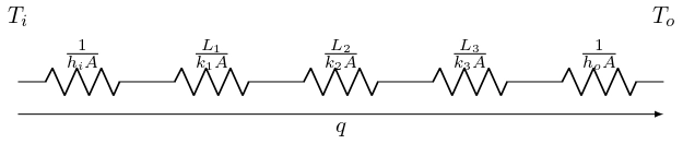
Thermal Resistance in the walls can be analyzed by splitting the wall into different section:
- The heat transfer between the fluid and the wall represents one thermal resistance (resistance due to convection).
- The resistance of the wall itself, based on its thickness and thermal conductivity, constitutes another thermal resistance.
- The heat transfer between the wall and the second fluid adds a third thermal resistance.
Also Read: Top 15 Fundamental Constants Every Chemical Engineer Should Know
Overall Heat Transfer Coefficient Table
In the real world, generally heat exchange takes place between material lies between two fluid masses. Here in the table below we are providing the values of overall heat transfer coefficient from various technical sources.
A high value of U represents that heat is being transferred efficiently through the system. It can be due to due to high thermal conductivity of the materials, effective heat transfer surfaces, or good convection conditions.
A low value of U represents heat transfer is less efficient. It could be due to poor thermal conductivity, inadequate surface area, or ineffective convection.
| Heat Exchange Configuration | U (W/m²K) |
|---|---|
| Walls and roofs dwellings with a 24 km/h outdoor wind: | |
| – Insulated roofs | 0.3–2 |
| – Finished masonry walls | 0.5–6 |
| – Frame walls | 0.3–5 |
| – Uninsulated roofs | 1.2–4 |
| Single-pane windows | ~ 6 |
| Air to heavy tars and oils | As low as 45 |
| Air to low-viscosity liquids | As high as 600 |
| Air to various gases | 60–550 |
| Steam or water to oil | 60–340 |
| Liquids in coils immersed in liquids | 110–2,000 |
| Feedwater heaters | 110–8,500 |
| Air condensers | 350–780 |
| Steam-jacketed, agitated vessels | 500–1,900 |
| Shell-and-tube ammonia condensers | 800–1,400 |
| Steam condensers with 25°C water | 1,500–5,000 |
| Condensing steam to high-pressure boiling water | 1,500–10,000 |
Source: A Heat Transfer Textbook, by John H. Lienhard V, Massachusetts Institute of Technology
Example Problem on Overall Heat Transfer Coefficient
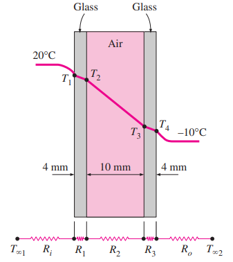
Consider a 0.8-m-high and 1.5-m-wide double-pane window consisting of two 4-mm-thick layers of glass \((k = 0.78 \, \text{W/m} \cdot ^\circ \text{C})\) separated by a 10-mm-wide stagnant air space \((k = 0.026 \, \text{W/m} \cdot ^\circ \text{C})\). Determine the steady rate of heat transfer through this double-pane window and the temperature of its inner surface for a day during which the room is maintained at \(20^\circ \text{C}\) while the temperature of the outdoors is \(10^\circ \text{C}\). Take the convection heat transfer coefficients on the inner and outer surfaces of the window to be \(h_1 = 10 \, \text{W/m}^2 \cdot ^\circ \text{C}\) and \(h_2 = 40 \, \text{W/m}^2 \cdot ^\circ \text{C}\), which includes the effects of radiation.
In the question given above we understand that rate of heat transfer
through the window and the inner surface temperature are to be determined.
The thermal resistance across the window pane can be split into different resistances are as follow:
- Convection resistance on the inner surface: \(R_i = R_{\text{conv,1}}\)
- Conduction resistance of the glass layers: \(R_1 = R_3 = R_{\text{glass}}\)
- Conduction resistance of the air gap: \(R_2 = R_{\text{air}}\)
- Convection resistance on the outer surface: \(R_o = R_{\text{conv,2}}\)
Area of the window, A = 0.8 m×1.5 m=1.2 m2
Now, calculating the values of thermal resistance one by one we get,
\(R_i = \frac{1}{h_1 \times A} \)
\(= \frac{1}{10 \, \text{W} \cdot \text{m}^{-2} \cdot \text{°C}^{-1} \times 1.2 \, \text{m}^2}\)
\( = \frac{1 \, \text{°C}}{12 \, \text{W}} = 0.08333 \, \frac{\text{°C}}{\text{W}}\)
\(R_1 = R_3 = \frac{L}{k_{\text{glass}} \times A}\)
\( = \frac{0.004 \, \text{m}}{0.78 \, \text{W} \cdot \text{m}^{-1} \cdot \text{°C}^{-1} \times 1.2 \, \text{m}^2}\)
\( = \frac{0.004 \, \text{m} \cdot \text{°C}}{0.936 \, \text{W} \cdot \text{m}} = 0.00427 \, \frac{\text{°C}}{\text{W}}\)
\(R_2 = \frac{L}{k_{\text{air}} \times A}\)
\(= \frac{0.01 \, \text{m}}{0.026 \, \text{W} \cdot \text{m}^{-1} \cdot \text{°C}^{-1} \times 1.2 \, \text{m}^2}\)
\(= \frac{0.01 \, \text{m} \cdot \text{°C}}{0.0312 \, \text{W} \cdot \text{m}} = 0.3205 \, \frac{\text{°C}}{\text{W}}\)
\(R_o = \frac{1}{h_2 \times A}\)
\(= \frac{1}{40 \, \text{W} \cdot \text{m}^{-2} \cdot \text{°C}^{-1} \times 1.2 \, \text{m}^2}\)
\(= \frac{1 \, \text{°C}}{48 \, \text{W}} = 0.02083 \, \frac{\text{°C}}{\text{W}}\)
Therefore, the total thermal resistance, across the window pane, as all are connected in series we get:
\(R_\text{total}\)=0.08333 +0.00427+0.3205+0.00427+0.02083
\(R_\text{total} = 0.4332 \frac{\text{°C}}{\text{W}}\)
The steady rate of heat transfer through the window is calculated using Fourier’s law:
\(\dot{Q} = \frac{\Delta T}{R_{\text{total}}}\)
here, \(\Delta T = T_{\text{inside}} – T_{\text{outside}}\)
\(\Delta T = 20°C− (-10°C) = 30°C\)
Substituting the values,
\(\dot{Q} = \frac{30 \, \text{°C}}{0.4332 \, \frac{\text{°C}}{\text{W}}} = 69.2 \text{W} \)
To find the inner surface temperature of the window, we use the following formula:
\(T_1 = T_{\text{ambient}} – Q \times R_{\text{conv,1}}\)
\(T_1 = 20^\circ \text{C} – (69.2 \times 0.08333 )\)
\(T_1 = 20^\circ \text{C} – 5.77^\circ \text{C} = 14.23^\circ \text{C}\)
Thus, the inner surface temperature of the window is approximately \( 14.2^\circ \text{C} \), we see the reduction in heat transfer due to high thermal resistance of the air layer between the glasses, which acts as an insulating barrier.
Also Read: Van der Waals Equation of State Calculator and PV Isotherms for Real Gases
Python Code for Overall Heat Transfer Coefficient
This Python code helps user to calculate the overall heat transfer coefficient U, the heat transfer rate Q, the temperature profile across a multi-layered wall, and the thermal resistances of each layer and the convective boundaries for unit Area.
Note: This Python code solves the specified problem. Users can copy the code and run it in a suitable Python environment. By adjusting the input parameters, users can observe how the output changes accordingly.
import numpy as np
import matplotlib.pyplot as plt
# Function to calculate the overall heat transfer coefficient U
def calculate_U(h_i, h_o, L1, k1, L2, k2, L3, k3):
U = 1 / (1/h_i + L1/k1 + L2/k2 + L3/k3 + 1/h_o)
return U
# Function to calculate the heat transfer rate Q
def calculate_Q(U, A, T1, T2):
Q = U * A * (T1 - T2)
return Q
# Function to calculate the temperature profile across the layers
def temperature_profile(T1, Q, h_i, h_o, L1, k1, L2, k2, L3, k3):
T_interface1 = T1 - Q * (1/h_i)
T_interface2 = T_interface1 - Q * (L1/k1)
T_interface3 = T_interface2 - Q * (L2/k2)
T2 = T_interface3 - Q * (L3/k3 + 1/h_o)
return [T1, T_interface1, T_interface2, T_interface3, T2]
# Function to calculate the thermal resistances
def calculate_resistances(h_i, h_o, L1, k1, L2, k2, L3, k3):
R_i = 1 / h_i
R1 = L1 / k1
R2 = L2 / k2
R3 = L3 / k3
R_o = 1 / h_o
return [R_i, R1, R2, R3, R_o]
# Given parameters
h_i = 50 # Heat transfer coefficient on the inside (W/m^2K)
h_o = 25 # Heat transfer coefficient on the outside (W/m^2K)
L1, k1 = 0.01, 1.0 # Thickness and thermal conductivity of layer 1 (m, W/mK)
L2, k2 = 0.02, 0.5 # Thickness and thermal conductivity of layer 2 (m, W/mK)
L3, k3 = 0.015, 0.8 # Thickness and thermal conductivity of layer 3 (m, W/mK)
A = 1 # Heat transfer area (m^2)
T1 = 100 # Temperature on the inside (°C)
T2 = 30 # Temperature on the outside (°C)
# Calculate the overall heat transfer coefficient U
U = calculate_U(h_i, h_o, L1, k1, L2, k2, L3, k3)
# Calculate the heat transfer rate Q
Q = calculate_Q(U, A, T1, T2)
# Calculate the temperature profile
temperatures = temperature_profile(T1, Q, h_i, h_o, L1, k1, L2, k2, L3, k3)
# Calculate the thermal resistances
resistances = calculate_resistances(h_i, h_o, L1, k1, L2, k2, L3, k3)
resistance_labels = ['R_i (inside)', 'R1', 'R2', 'R3', 'R_o (outside)']
# Distance points for the temperature profile plot (cumulative thicknesses)
distances = [0, L1, L1+L2, L1+L2+L3, L1+L2+L3+0.01] # Add small value for the last layer for plotting
# Print the results
print(f"Overall Heat Transfer Coefficient (U): {U:.4f} W/m^2K")
print(f"Heat Transfer Rate (Q): {Q:.2f} W")
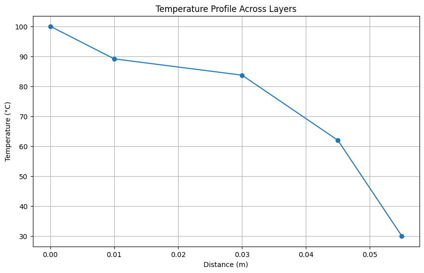
# Plotting the temperature profile
plt.figure(figsize=(8, 6))
plt.plot(distances, temperatures, marker='o')
plt.xlabel('Distance (m)')
plt.ylabel('Temperature (°C)')
plt.title('Temperature Profile Across Layers')
plt.grid(True)
plt.show()
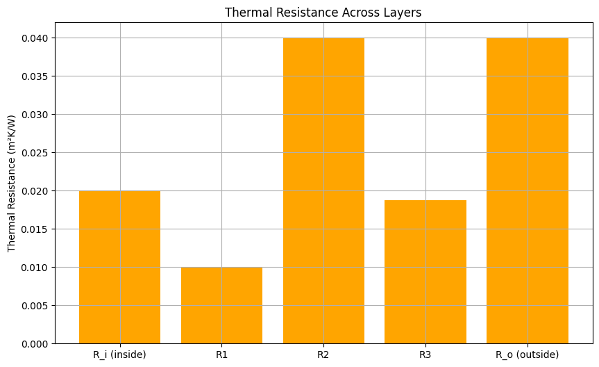
# Plotting the thermal resistances
plt.figure(figsize=(8, 6))
plt.bar(resistance_labels, resistances, color='orange')
plt.ylabel('Thermal Resistance (m²K/W)')
plt.title('Thermal Resistance Across Layers')
plt.grid(True)
plt.show()Output:
- Overall Heat Transfer Coefficient (U): 7.7670 W/m2K
- Heat Transfer Rate (Q): 543.69 W
Resources
- Heat Transfer a Practical Approach – Book by Yunus A Çengel
- “Fundamentals of Heat and Mass Transfer” by Theodore L. Bergman, Adrienne S. Lavine, Frank P. Incropera, and David P. DeWitt.
- “Heat Transfer Book” by David W. Hahn.
- “Conduction of Heat in Solids” by H.S. Carslaw and J.C. Jaeger.
- “Introduction to Heat Transfer” by Frank P. Incropera, David P. DeWitt, Theodore L. Bergman, and Adrienne S. Lavine.
Disclaimer: The Solver provided here is for educational purposes. While efforts ensure accuracy, results may not always reflect real-world scenarios. Verify results with other sources and consult professionals for critical applications. Contact us for any suggestions or corrections.