Heat Conduction in Cylindrical Systems – Online Calculator & Python Code

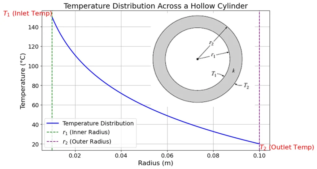
Heat transfer through conduction in cylindrical coordinates has direct application in pipes, tubes, and cylindrical structures such as boilers, heat exchangers, and insulation materials. In cylindrical systems, heat conduction occurs from a higher temperature at the inner radius to a lower temperature at the outer radius.

In cylindrical conduction the heat flow is not uniform because of changing area as the radius varies. This radially varying area gives a logarithmic temperature profile across the cylinder’s thickness, which makes the analysis more complex when compared to plane walls.

Related: Heat Transfer through Convection Calculator – Newton’s Law of Cooling

Related: Heat Transfer through Conduction Calculator – Fourier’s law

Heat Conduction Equation in Cylindrical Coordinates

For steady-state heat conduction in a cylindrical wall without internal heat generation, Fourier’s law of heat conduction in cylindrical coordinates is given by:

\[q = -k A \frac{dT}{dr}\]

where:

• \( q \) is the heat transfer rate,
• \( k \) is the thermal conductivity of the material,
• \( A \) is the area through which heat is transferred (for a cylindrical shell, \( A = 2 \pi r L \), where L is the length of the cylinder),
• \( \frac{dT}{dr} \) is the temperature gradient in the radial direction.

Related: Overall Heat Transfer Coefficient Calculator for Composite Walls

In cylindrical coordinates, heat flows through an area that changes with radius r. This changing area impacts how heat is distributed, leading to a temperature gradient that is not linear but logarithmic.

The heat transfer rate across a cylindrical wall, based on the temperature difference and material properties, is:

\[q = \frac{2 \pi k L (T_1 – T_2)}{\ln\left(\frac{r_2}{r_1}\right)}\]

where in S.I units,

• k is the Thermal conductivity of the material (W/m·K)
• T₁ is the temperature at the inner surface of the cylinder (K)
• T₂ is the temperature at the outer surface of the cylinder (K)
• r₁ is the Inner radius of the cylinder (m)
• r₂ is the Outer radius of the cylinder (m)

Note: This cylindrical conduction equation applies to steady-state heat transfer in hollow cylinders, assuming constant thermal conductivity and no internal heat generation.

Related: Critical Thickness of Insulation Calculator for Cylinder and Sphere

Heat Conduction in Cylinder Calculator

The Heat Conduction in Cylinder Calculator is a user-friendly tool designed to calculate key parameters related to heat transfer in cylindrical systems. Users can select which parameter to be calculated by choosing from a dropdown menu and putting the required input parameters to get the result.

Related: Heat Transfer through Convection Calculator – Newton’s Law of Cooling

Related: Convection Cooling Time of a Sphere Calculator using Lumped Capacitance Method

Related: Heat Conduction in Spherical Shell – Online Calculator & Python Code

Derivation for Heat Conduction in Cylinder

To derive the heat transfer through conduction in cylindrical coordinates, consider a hollow cylinder with inner radius (r₁) outer radius (r₂) inner surface temperature (T₁), and outer surface temperature (T₂). Heat flows radially outward, and we assume steady-state conduction with no internal heat generation.

From the Fourier’s law of heat conduction states:

\[q = -k A \frac{dT}{dr}\]

In cylindrical coordinates, the lateral surface area ( A ) through which heat flows at a radius ( r ) over the cylinder length ( L ) is:

\[A = 2 \pi r L\]

Substituting this into Fourier’s law, we get:

\[q = -k (2 \pi r L) \frac{dT}{dr}\]

or,

\[\frac{dT}{dr} = -\frac{q}{2 \pi k L \cdot r}\]

Now, separating variables and rearrange the equation

\[\int_{T_1}^{T_2} dT = -\int_{r_1}^{r_2} \frac{q}{2 \pi k L \cdot r} \, dr\]

Integrating the left side with respect to T from T₁ to T₂ and the right side with respect to r from r₁ to r₂ :

\[T_2 – T_1 = -\frac{q}{2 \pi k L} \int_{r_1}^{r_2} \frac{1}{r} \, dr\]

The integral of \( \frac{1}{r} \) with respect to ( r ) is \( \ln(r) \), so we have:

\[T_2 – T_1 = -\frac{q}{2 \pi k L} \ln\left(\frac{r_2}{r_1}\right)\]

This equation represents the temperature profile at any radial position r follows a logarithmic profile across the cylinder’s thickness.

Further rearranging above equation, the heat Transfer Rate (q) equation is given as:

\[q = \frac{2 \pi k L (T_1 – T_2)}{\ln\left(\frac{r_2}{r_1}\right)}\]

This is the expression for analyzing radial heat conduction in cylindrical systems, such as pipes, insulation layers, and various cylindrical thermal devices.

In terms of thermal resistance ( R ) for radial conduction in a cylindrical wall is defined as:

\[R = \frac{\ln\left(\frac{r_2}{r_1}\right)}{2 \pi k L}\]

Then, the heat transfer rate can be rewritten as:

\[q = \frac{T_1 – T_2}{R}\]

For this relatively thick pipe wall for the cylindrical geometry in heat transfer analysis, heat transfer coefficient can be calculated by equating the expression \(Q = h_{\text{wall}} \cdot A \cdot (T_i – T_o)\) where \(A = 2 \pi r_i L \) is the area based on the inner diameter.

\[h_{\text{wall}} = \frac{2k}{d_{\text{i}} \ln(d_{\text{o}}/d_{\text{i}})}\]

where (d_i = 2r_i ) and ( d_o = 2r_o ) are the inner and outer diameters of the pipe.

Note: If the heat flux is based on the inner diameter and the pipe wall is thin, the wall curvature is negligible, then it considered as flat or plane wall. There simplifies the heat transfer coefficient calculation to h_wall=2k/L​.

Related: Heat Transfer Calculators for Chemical Engineering

Related: Fluid Mechanics Calculators for Chemical Engineering

Example Problem on Heat Conduction in Cylinder

Given Data:

• Outside diameter of pipe, D = 30 cm = 0.3 m
• Surface temperature of pipe, T_s​ = 220°C
• Surrounding temperature, T_∞​ = 25°C
• Convective heat transfer coefficient, h = 22 W/m²K
• Stefan – Boltzmann Constant, σ = 5.67×10⁻⁸ W/m²K⁴
• Length. L = 1 m

considering the bare pipe, heat lost over the surface, Q = heat convected + heat radiated

Q = h A (∆T) + σA(T₁⁴ – T₂⁴)

Q = 22 × π × 0.3 × 1(220 – 25) + 5.67 × 10^-8 x π × 0.3 {(220 + 273)⁴ – (25 + 273)⁴}

Q = 4043.23 + 2735.34 = 6778.57 W/m length.

To find the unknown surface temperature ( T ), energy balance is needed, where the heat conducted through the pipe wall equals the heat lost by convection and radiation.

The equation can be written as Heat Conduction = Heat Convection + Heat Radiation:

Related: Thermal Radiation – Stefan Boltzmann Law Calculator

\[\frac{(T – 220)}{\ln\left(\frac{0.36}{0.225}\right) \times 2 \pi \times 0.36}\]

\[ = 22 \times \pi \times 0.45 \times (T – 298) +\]

\[5.67 \cdot 10^{-8} \cdot \pi \cdot 0.45 \left( \left( \frac{T}{100} \right)^4 – \left( \frac{298}{100} \right)^4 \right)\]

This equation can be solved for ( T ) using a numerical method, such as the Newton-Raphson method or using a Python script with scipy.optimize.fsolve.

import numpy as np
from scipy.optimize import fsolve

# Constants
T1 = 273 + 220  # Equivalent to 493
ln_term = np.log(0.225 / 0.015)
pi = np.pi
constant1 = 2 * pi * 0.36
constant2 = 22 * pi * 0.45
constant3 = 5.67 * pi * 0.45
T_ref = 298

# Define the equation as a function
def equation(T):
    left_side = (T1 - T) / ln_term * constant1
    right_side = constant2 * (T - T_ref) + constant3 * ((T / 100)**4 - (T_ref / 100)**4)
    return left_side - right_side

# Initial guess for T
T_initial_guess = 300

# Solving for T
T_solution = fsolve(equation, T_initial_guess)

print(f"The solution for T is approximately: {T_solution[0]:.2f} K")

Output: The surface temperature T is approximately: 302.01 K

Therefore the temperature on the surface is 302.01 K.

Related: Joule-Thomson Effect – Coefficient Calculation for CO2 and N2

Related: Nusselt Number Calculator – Significance and Calculation

Python Code Heat Conduction in Cylinder

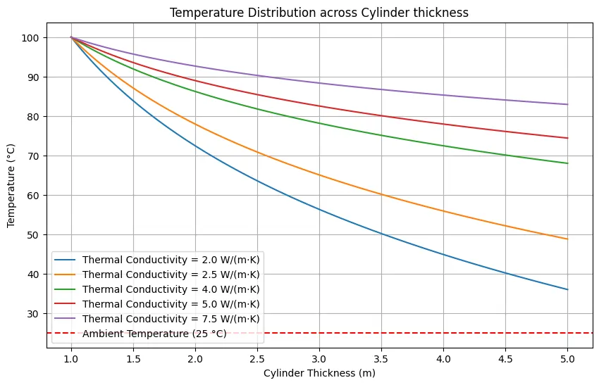
This python code helps user to compute the temperature distribution in a cylindrical object under steady-state heat conduction with no heat generation. it then calculates the temperature at different radial positions within the cylinder which is shown in the plot.

Note: This Python code solves the specified problem. Users can copy the code and run it in a suitable Python environment. By adjusting the input parameters, users can observe how the output changes accordingly.

import numpy as np
import matplotlib.pyplot as plt

def temperature_distribution(r1, r2, q, thermal_conductivity, length):
    """
    Calculate the temperature at radius r2 given the heat flux q in a cylindrical shell.
    
    Parameters:
    - r1 (float): Inner radius of the cylinder (m)
    - r2 (float): Radius at which temperature is calculated (m)
    - q (float): Heat flux (W/m)
    - thermal_conductivity (float): Thermal conductivity (W/(m·K))
    - length (float): Length of the cylinder (m)
    
    Returns:
    - T2 (float): Temperature at radius r2 (°C)
    """
    T1 = 100  # Inner temperature (°C)
    T2 = T1 - (q / (2 * np.pi * thermal_conductivity * length)) * np.log(r2 / r1)
    return T2

# Parameters
inner_radius = 1.0  # Inner radius of the cylinder (m)
outer_radius = 5.0  # Outer radius of the cylinder (m)
length = 1.0  # Length of the cylinder (m)
heat_flux = 500  # Heat flux (W/m)

# Different thermal conductivities
thermal_conductivities = [2.0, 2.5, 4.0, 5.0, 10.0]  # W/(m·K)

# Radial positions
radii = np.linspace(inner_radius, outer_radius, 100)

# Plotting
plt.figure(figsize=(10, 6))

for k in thermal_conductivities:
    T2 = [temperature_distribution(inner_radius, r, heat_flux, k, length) for r in radii]
    plt.plot(radii, T2, label=f'Thermal Conductivity = {k} W/(m·K)')

plt.title('Temperature Distribution in a Cylinder with Varying Thermal Conductivity')
plt.xlabel('Radius (m)')
plt.ylabel('Temperature (°C)')
plt.axhline(y=25, color='r', linestyle='--', label='Ambient Temperature (25 °C)')  # Outer temperature
plt.legend()
plt.grid()
plt.show()

Output:

Resources

• Heat Transfer a Practical Approach – Book by Yunus A Çengel
• “Fundamentals of Heat and Mass Transfer” by Theodore L. Bergman, Adrienne S. Lavine, Frank P. Incropera, and David P. DeWitt.
• “Heat Transfer Book” by David W. Hahn.
• “Conduction of Heat in Solids” by H.S. Carslaw and J.C. Jaeger.
• “Introduction to Heat Transfer” by Frank P. Incropera, David P. DeWitt, Theodore L. Bergman, and Adrienne S. Lavine.

Disclaimer: The Solver provided here is for educational purposes. While efforts ensure accuracy, results may not always reflect real-world scenarios. Verify results with other sources and consult professionals for critical applications. Contact us for any suggestions or corrections.