Table of Contents
When fluid flows through a pipe or channel, friction factor calculates the resistance that fluid faces due to factors like surface roughness or flow velocity which impacts the pressure drop and energy efficiency. Moody’s Diagram are the important tool to determine the friction factor in both smooth and rough pipes.
Smooth pipes, like those made of glass or plastic, have lower friction factors due to lesser surface irregularities, while rough pipes, such as those made of cast iron, have higher friction factors due to higher surface roughness.
Related: Newton’s Law of Viscosity Calculator – Dynamic Viscosity
Moody Chart Calculator
This Friction Factor Calculator helps user to determine the friction factor for both smooth and rough pipes for different flow regimes based on the Reynolds number.
For smooth pipes, the calculator uses the Blasius equation for turbulent flow, while for rough pipes, it applies the Colebrook-White equation, requiring relative roughness.
Related: Bernoulli’s Equation Calculator / Solver – Interactive Python Code
Related: Stoke’s Law Calculator for Terminal Velocity – Derivation and Python Code
Moody’s Diagram / Moody’s Chart
The Moody diagram (or Moody chart) is a log – log plot between three variables Reynolds Number, Relative Roughness and Friction Factor. This diagram is useful in fluid mechanics to determine the for flow in a pipe.
Moody’s Diagram is a graphical tool used in fluid mechanics to determine the Darcy-Weisbach friction factor \((f)\), which is essential in calculating the pressure drop or head loss due to friction in pipe flow.
Related: Head Loss or Pressure Loss Calculator using Darcy-Weisbach Equation

Download python code to plot the Moody’s Diagram – click here
Related: Froude Number Calculator – Significance and Applications
To understand the Moody’s diagram the graph is plotted for three different regimes of Reynolds Number i.e Laminar Flow, Transitional Flow or Turbulent Flow.
| Flow Region | Condition | Description |
|---|---|---|
| Laminar Flow | Re<2,300 | The flow is laminar, and the friction factor is calculated using f=64/Re. This region is shown by a straight line on the chart. |
| Turbulent Flow | Re>4,000 | The flow becomes turbulent, and the friction factor depends on both the Reynolds number and the relative roughness ϵ/D. |
| Turbulent – Smooth Pipes | Re>4,000 | For smooth pipes (low relative roughness), the friction factor decreases as the Reynolds number increases. |
| Turbulent – Rough Pipes | Re>4,000 | For rough pipes (higher ϵ/D), the friction factor levels off and becomes independent of the Reynolds number at high values (fully rough flow). |
| Transition Flow | 2,300<Re<4,000 | The transition zone is where the flow characteristics are unpredictable, and the friction factor changes fastly. |
Related: Read More about Dimensionless Number
What is the Darcy Friction Factor?
The friction factor \(f\) also known as Darcy-Weisbach Friction Factor is a dimensionless quantity that represents the frictional resistance or energy loss due to shear forces between fluid layers as the fluid flows through a pipe or channel.
There is another form of friction factor known as Fanning Friction Factor \((f_F)\) which is typically 1/4th of the Darcy friction factor \((f_F=\frac{f}{4})\) used in different industries.
Friction Factor depends on the Reynolds number (Re) and the relative roughness of the pipe. Applicable equation and ranges are shown in table given below:
| Flow Type | Reynolds Number (Re) | Pipe Type | Equation Used |
|---|---|---|---|
| Laminar Flow | Re < 2000 | Smooth & Rough | \(f = \frac{64}{Re}\) |
| Turbulent Flow | 2000 < Re < 4000 | Smooth & Rough | Unpredictable (transitional region) |
| Turbulent Flow | 4000 < Re < 100,000 | Smooth Pipe | (Blasius Equation) \(f = 0.3164 \cdot Re^{-0.25}\) |
| Turbulent Flow | Re > 4000 | Rough Pipe | Colebrook-White Equation |
Related: Head Loss or Pressure Loss Calculator using Darcy-Weisbach Equation
Related: Centrifugal Pump Sizing Calculation – TDH, NPSHa vs Flow Rate curve & Power Required
Colebrook-White Equation
The Colebrook-White equation is an empirical formula used to determine the Darcy-Weisbach friction factor \((f)\) for turbulent flow in a pipe. The equation is implicit and cannot be solved algebraically for \(f\), therefore requires iterative methods or numerical solution.
Colebrook-White equation combines both the effect of pipe roughness and the Reynolds number on friction losses and written as:
\[\frac{1}{\sqrt{f}} = -2 \log \left( \frac{\varepsilon/D}{3.7} + \frac{2.51}{Re \sqrt{f}} \right)\]
where:
- \( f \) is the Darcy-Weisbach friction factor (dimensionless),
- ε/D is the relative roughness represents the roughness of the pipe’s surface relative to its diameter.
- D is the pipe diameter (m),
- Re is the Reynolds number (dimensionless),
- log is the logarithm to base 10.
- The Colebrook-White equation is applicable for turbulent flow (Re>4000) in both smooth and rough pipes.
- The Moody’s diagram or Moody’s chart uses the Colebrook-White equation for turbulent flow
Here are the common values of roughness used in various Industries:
| Pipe Material | Roughness (ϵ) (mm) |
|---|---|
| Glass, Brass, Copper, Lead (Smooth) | Smooth (Negligible) |
| Steel, Wrought Iron | 0.045 |
| Asphalted Cast Iron | 0.12 |
| Galvanized Iron | 0.15 |
| Cast Iron | 0.26 |
| Concrete | 0.30 to 3.0 |
| Riveted Steel | 0.90 to 9.0 |
Also Read: Area of Cross-Section Calculator for Hollow Sections, Beams & Shapes

Swamee-Jain Equation
The Colebrook-White equation is implicit – the friction factor appears on both sides, so it has to be solved iteratively. Swamee and Jain published an explicit approximation in 1976 that avoids the iteration entirely:
\[f = \frac{0.25}{\left[ \log_{10}\left( \frac{\varepsilon/D}{3.7} + \frac{5.74}{Re^{0.9}} \right) \right]^2}\]
where ε/D is the relative roughness and Re the Reynolds number.
Because it is explicit, it can be evaluated directly in a spreadsheet or by hand, which is why it appears in most piping design references.
Validity: 10⁻⁶ ≤ ε/D ≤ 10⁻² and 5000 ≤ Re ≤ 10⁸. Within this window it agrees with Colebrook-White to within about 1–3%; checked across the full Moody chart, the largest deviation is close to 3%. For most engineering work that difference is smaller than the uncertainty in the roughness value itself.
Haaland Equation
Haaland proposed a similar explicit approximation in 1983, arranged so the friction factor can be found in a single step:
\[\frac{1}{\sqrt{f}} = -1.8 \log_{10}\left[ \left( \frac{\varepsilon/D}{3.7} \right)^{1.11} + \frac{6.9}{Re} \right]\]
The 1.11 exponent is what lets a single logarithm reproduce the shape of the Colebrook curve so closely.
Validity: turbulent flow, roughly 4000 < Re < 10⁸. It is typically quoted as accurate to within 2% of Colebrook-White, and is slightly closer than Swamee-Jain across most of the chart — measured over the full range, its worst deviation is about 1.3%.
Which should you use? Colebrook-White is the reference and what the Moody chart is drawn from – use it when accuracy matters. Swamee-Jain and Haaland are for when you need a direct calculation without iteration. All three are available in the calculator above, so you can switch between them and see the difference for your own case.
Blasius Equation
The Blasius equation is an empirical formula used to estimate the friction factor in smooth pipes for turbulent flow. The correlation is written as:
\[f = \frac{0.0791}{Re^{0.25}}\]
where:
- \( f \) is the Darcy-Weisbach friction factor (dimensionless),
- Re is the Reynolds number (dimensionless).
- The Blasius equation is only applicable to smooth pipes and for Reynolds numbers ranging between 4000 and 100,000.
- The Blasius equation is a simplified case of the Colebrook-White equation
Related: Hagen-Poiseuille Equation Calculator / Poiseuille’s Law Solver
Example Problem on solving friction factor
In a laboratory, the water supply is drawn from a roof storage tank 25 m above the water discharge point. If the friction factor is 0.008, the pipe diameter is 5 cm and the pipe is assumed vertical, calculate the maximum volume of flow achievable, if separation losses are ignored.
Given:
- Head of water available, H = 25 m
- Diameter of pipe, D = 5 cm = 0.05 m
- Friction factor for the pipe, f = 0.008
- Length of the pipe, L = 25 m
- g = 9.81 m/s2
first, calculating the cross-sectional area of the pipe, A is:
\[A = \frac{\pi D^2}{4} = \frac{\pi (0.05)^2}{4} \]
\[A = 1.964286 \times 10^{-3 } \, \text{m}^2\]
Head lost due to pipe friction, hf is:
\[h_f = H = 25 \, \text{m}\]
Using the Darcy-Weisbach equation for head loss due to pipe friction:
\[h_f = \frac{f L V^2}{2g D}\]
Substituting the given values:
\[25 = \frac{0.008 \cdot 25 \cdot V^2}{2 \cdot 9.81 \cdot 0.05}\]
solving for V, we get
\[V^2 = 30.65625\]
\[V = \sqrt{30.65625} = 5.53 \, \text{m/s}\]
Now, calculating the flow rate, Q
\[Q = A \cdot V = (1.964286 \times 10^{-3} \cdot (5.53)\]
\[Q = 0.010876 \, \text{m}^3/\text{s}\]
Thus, the maximum volume of flow achievable is approximately \(0.010876 \, m^3/s \).
Related: Weber Number Calculator – Significance and Calculation

Python Code to Calculate Friction Factor
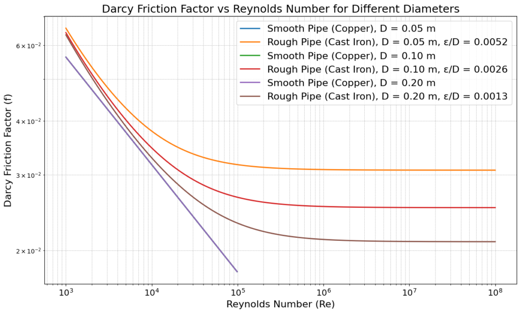
This Python code helps user to calculate and visualize the Darcy friction factor for smooth and rough pipes based on the Reynolds number for different pipe diameter. We have used the conditions on Moody’s diagram for different flow regimes.
Note: This Python code solves the specified problem. Users can copy the code and run it in a suitable Python environment. By adjusting the input parameters, and observe how the output changes accordingly.
import numpy as np
import matplotlib.pyplot as plt
from scipy.optimize import fsolve

# Define the Colebrook-White equation for rough pipes
def colebrook_white(f, Re, rel_roughness):
    return 1/np.sqrt(f) + 2*np.log10(rel_roughness/3.7 + 2.51/(Re*np.sqrt(f)))

# Define the Blasius equation for smooth pipes (valid for Re < 100,000)
def blasius(Re):
    return 0.3164 / (Re ** 0.25)

# Define function to compute friction factor for rough pipes using Colebrook-White
def friction_factor_rough(Re, rel_roughness):
    f_initial = 0.02  # Initial guess
    f_solution = fsolve(colebrook_white, f_initial, args=(Re, rel_roughness))
    return f_solution[0]

# Define diameters for both smooth and rough pipes
diameters = [0.05, 0.1, 0.2]  # Diameters in meters (e.g., 50mm, 100mm, 200mm)

# Roughness for cast iron pipes (rough pipe)
epsilon_cast_iron = 0.00026  # in meters (0.26 mm)

# Reynolds numbers range
Re_range = np.logspace(3, 8, 500)  # From 1,000 to 100,000,000

# Plot friction factors for each diameter
plt.figure(figsize=(14, 8))

for D in diameters:
    # Compute relative roughness for cast iron pipes
    rel_roughness = epsilon_cast_iron / D

    # Compute friction factor for smooth copper pipes (Blasius equation)
    f_smooth = [blasius(Re) if Re < 100000 else np.nan for Re in Re_range]

    # Compute friction factor for rough cast iron pipes (Colebrook-White equation)
    f_rough = [friction_factor_rough(Re, rel_roughness) for Re in Re_range]

    # Plot smooth pipe (copper)
    plt.loglog(Re_range, f_smooth, label=f'Smooth Pipe (Copper), D = {D:.2f} m', lw=2)

    # Plot rough pipe (cast iron)
    plt.loglog(Re_range, f_rough, label=f'Rough Pipe (Cast Iron), D = {D:.2f} m, ε/D = {rel_roughness:.4f}', lw=2)

# Add labels, title, and legend
plt.title('Darcy Friction Factor vs Reynolds Number for Different Diameters')
plt.xlabel('Reynolds Number (Re)')
plt.ylabel('Darcy Friction Factor (f)')
plt.legend(loc='best')
plt.grid(True, which='both', linestyle='--', linewidth=0.8)

# Show the plot
plt.show()
Output:
Resources
- “Fluid Mechanics” by Frank M. White
- “Introduction to Fluid Mechanics” by Robert W. Fox, Alan T. McDonald, and Philip J. Pritchard
- “Principles of Heat and Mass Transfer” by Frank P. Incropera and David P. DeWitt
- Python.org – The official Python website offers tutorials, documentation, and resources for learning Python.
Disclaimer: The Solver provided here is for educational purposes. While efforts ensure accuracy, results may not always reflect real-world scenarios. Verify results with other sources and consult professionals for critical applications. Contact us for any suggestions or corrections.








This is a fantastic breakdown of using Moody’s Diagram! I appreciate the clarity in explaining how to differentiate between smooth and rough pipes. The friction factor calculator links are incredibly helpful for practical applications. Looking forward to more posts like this!