Thermal Boundary Layer Thickness (δT) for Flat Plate

What is Thermal Boundary Layer Thickness?

The Thermal Boundary Layer is a concept in fluid dynamics and heat transfer that describes the region of fluid near to the solid surface where temperature gradients exist due to thermal interaction between the fluid and the surface. This layer is characterized by a change from the temperature of the solid surface to the bulk temperature of the fluid. The thickness of this layer, typically denoted as \(\delta_{T}\).

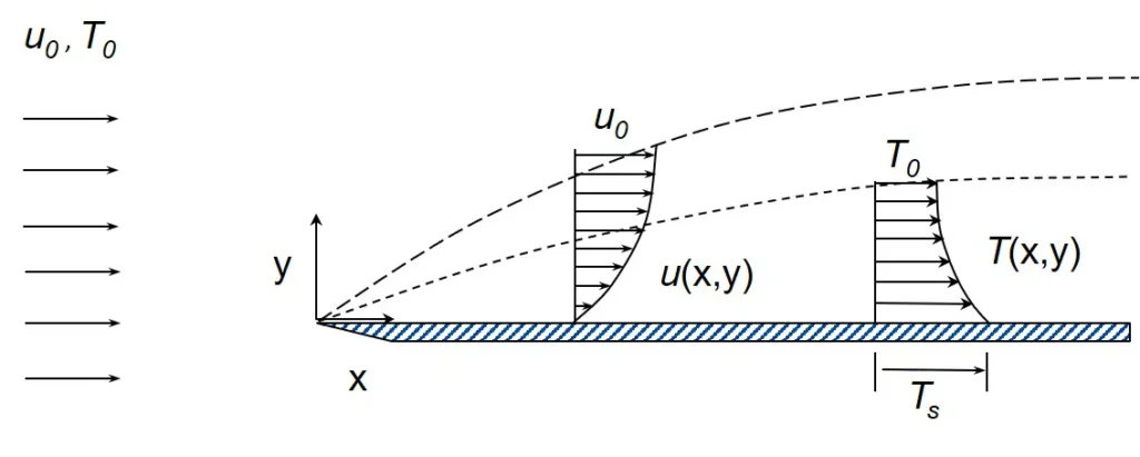
Image Source: wikipedia – Thermal Boundary Layer

Thermal Boundary Layer Thickness, \(\delta_{T}\) is defined as the distance from the body at which the temperature reaches 99% of the free-stream temperature (from an inviscid region) i.e the distance in y direction at which the ratio \(\left( \frac{T_s – T}{T_s – T_\infty} \right) = 0.99\).

Related: Convective Heat Transfer Calculator – Newton’s law of cooling

Related: Reynolds Number Calculator for a Circular Pipe

Thermal Boundary Layer Thickness For Laminar Flow

For the laminar flow (where \(Re < 5 \times {10^5}\)) the fluid is well-ordered, with smooth and regular streamlines, and the velocity at any point remains constant. No macroscopic mixing occurs between layers, and momentum and heat transfer occur mainly through molecular diffusion.

For laminar flow over a flat plate at zero incidence, the thermal boundary layer thickness is given by:

\[\delta_T = \delta_v \mathrm{Pr}^{-1/3}\] — (1)

From Blasius velocity boundary layer thickness, \(\delta_v\)

\[\delta_v = 5.0 \frac{x}{\sqrt{Re_x}} = 5.0 \sqrt{\frac{\nu x}{u_0}}\]

Now, replacing the value of \(\delta_v\) into equation 1, we get

\[\delta_T = 5.0 \sqrt{\frac{\nu x}{u_0}} \mathrm{Pr}^{-1/3}\]

where

• \(\mathrm{Pr}\) is the Prandtl number,
• \(\delta_v\) is the thickness of the velocity boundary layer,
• \(u_0\) is the freestream velocity,
• \(x\) is the distance downstream from the start of the boundary layer,
• \(\nu\) is the kinematic viscosity.

For different substances, with different Prandtl Numbers, the thermal boundary layer thickness is different. For example with the help of table given below:

Fluid	Kinematic Viscosity (m²/s)	Prandtl Number
Air	16.960 × 10⁻⁶	0.699
Carbon dioxide	9.294 × 10⁻⁶	0.76
Hydrogen	118.600 × 10⁻⁶	0.684
Water	0.657 × 10⁻⁶	4.34
Mercury	0.109 × 10⁻⁶	0.0252
Glycerine	223.000 × 10⁻⁶	2450

Here, we will calculate the Hydrodynamic Boundary layer thickness, \(\delta_v\) for Reynold’s number in the laminar region (assuming \(Re = 10^5\)) using formula \(\delta_v = 5.0 \frac{x}{\sqrt{Re_x}}\).

Based on the values of \(\delta_v\), thermal boundary layer thickness \(\delta_T\) using equation 1(mentioned above)

The calculation table is provided below:

Fluid	\(x\) at Re =105	\(\delta_v\)(for Re = 105), mm	\(\delta_T\) (for Re = 105), mm
Air	0.57	8.94	10.06
Carbon dioxide	0.31	4.90	5.36
Hydrogen	3.95	62.51	70.85
Water	0.02	0.35	0.21
Mercury	0.0036	0.06	0.19
Glycerine	7.43	117.53	8.95

Now, plotting the graph from the given data, we see:

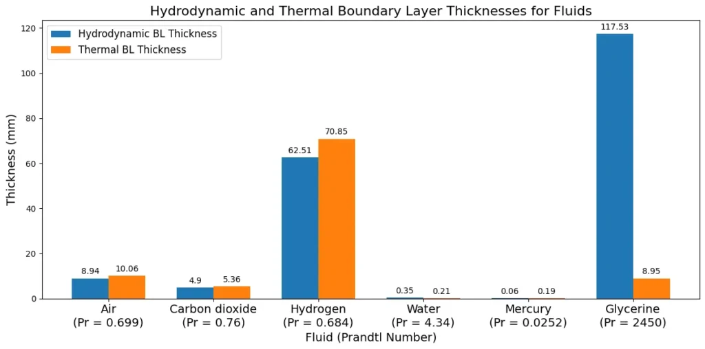
From the plot, we understand the relation between Hydrodynamic and Thermal boundary layer thickness at different Prandtl Number.

For Case 1: If \( \text{Pr} = 1 \), i.e \(\delta_t = \delta_v\)

The thermal boundary layer thickness (\( \delta_t \)) at any position ( x ) is equal to the hydrodynamic boundary layer thickness (\( \delta_v \)).

For Case 2: If \( \text{Pr} < 1 \), i.e \(\delta_t < \delta_v\)

The thermal boundary layer thickness (\( \delta_t \)) at any position ( x ) is thicker than the hydrodynamic boundary layer thickness (\( \delta_v \)).

For Case 3: If \( \text{Pr} > 1 \), i.e \(\delta_t > \delta_v\)

The thermal boundary layer thickness (\( \delta_t \)) at any position ( x ) is thinner than the hydrodynamic boundary layer thickness (\( \delta_v \)).

Also Read: Chemical Engineering as a career option in India

Thermal Boundary Layer Thickness For Turbulent Flow

For the turbulent flow (where \(Re \geq 5 \times {10^5}\)) over a flat plate, Large particles of the fluid moves from one layer to another and motion of particles become irregular.

The thermal boundary layer thickness (\(\delta_{T}\)) formed is not determined by the thermal diffusion but due to the random fluctuations in the outer region of the fluid boundary layer. Therefore, it’s determined by the Reynolds number, not the Prandtl number.

\[\delta_{T} \approx \delta \approx 0.37\frac{x}{{\mathrm{Re}}_{x}^{1/5}}\]

where \(Re_x = \frac{u_0 x}{\nu}\) represents the Reynolds number.

This turbulent boundary layer thickness formula assumes:

1. The flow is turbulent right from the start of the boundary layer.
2. The turbulent boundary layer behaves in a geometrically similar manner.

Related: 10 Mostly used Dimensionless Numbers in Chemical Engineering

Example Problem on Thermal Boundary Layer Thickness

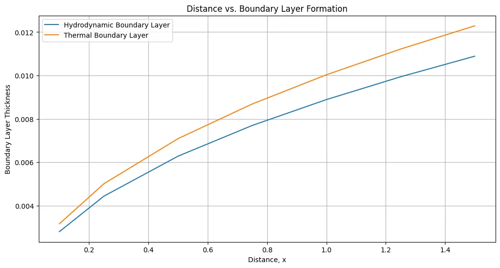
Air at \(20^\circ \text{C}\) and one atmosphere flows over a surface at \(100^\circ \text{C}\) with a free stream velocity of \(6 \, \text{m/s}\). Determine the values of Reynolds number, thermal and hydrodynamic boundary layer thicknesses at distances of \(0.1\), \(0.25\), \(0.5\), \(0.75\), \(1\), \(1.25\) \(m\) from the leading edge. Also, determine the length at which the flow turns to turbulent, taking the critical Reynolds number as \(5 \times 10^5\).

Given,

• \(\nu = 18.97 \times 10^{-6} \text{m}^2/\text{s}\),
• \(Pr = 0.696\),
• \(u_0 = 6 \, \text{m/s}\)

Firstly, calculating the values of \(Re_x\) for the given distance \(x\) from the leading edge using formula \(Re_x = \frac{u_0 x}{\nu}\).

Then calculating \(\delta_v\) using \(\delta_v = 5.0 \frac{x}{\sqrt{Re_x}}\).

Then calculating and \(\delta_T\) using \(\delta_T = \delta_v \mathrm{Pr}^{-1/3}\)

The calculation table is provided below based on the given distance from the leading edge.

Distance \(x\)	\(Re_x\)	\(\delta_v\) , mm	\(\delta_T\), mm
0.10	31628.9	2.811	3.17
0.25	79072.2	4.445	5.01
0.50	158144.4	6.287	7.09
0.75	237216.7	7.699	8.68
1.00	316288.9	8.891	10.02
1.25	395361.1	9.940	11.20
1.50	474433.3	10.889	12.27

To determine the length at which the flow turns to turbulent, taking the critical Reynolds number as \(5 \times 10^5\), using Reynolds number formula \(Re_x = \frac{u_0 x}{\nu}\)

\(5 \times {10^5} = \frac{6 x}{18.97 \times 10^{-6}}\)

\(x = 1.58 \) mm

Therefore, the fluid will turns to be turbulent at a length of 1.58 mm from the leading edge.

Resources

1. “Principles of Heat Transfer” by Frank Kreith and Raj M. Manglik
2. “Fundamentals of Heat and Mass Transfer” by C.P. Kothandaraman
3. “Introduction to Heat Transfer” by Theodore L. Bergman, Adrienne S. Lavine, Frank P. Incropera, and David P. DeWitt
4. “Python Documentation” – Official guides and references for Python.

Disclaimer: The Solver provided here is for educational purposes. While efforts ensure accuracy, results may not always reflect real-world scenarios. Verify results with other sources and consult professionals for critical applications. Contact us for any suggestions or corrections.