Joule-Thomson Effect – Coefficient Calculation for CO2 and N2

What is Joule-Thomson Effect

The Joule-Thomson effect is a thermodynamic process (also known as Joule–Kelvin effect or Kelvin–Joule effect) that describes the temperature change of a real gas (as opposed to an ideal gas) when it is forced through a valve or porous plug while kept insulated so that no heat is exchanged with the environment. This process is known as a throttling process or Joule-Thomson expansion.

In simpler terms Joule-Thomson effect occurs when the expansion of fluid takes place from high pressure to low pressure at constant enthalpy, then it shows the temperature change. The approximation to take place such process in real world by providing an expansion of fluid from high pressure to low pressure across a valve or orifice or porous medium. 

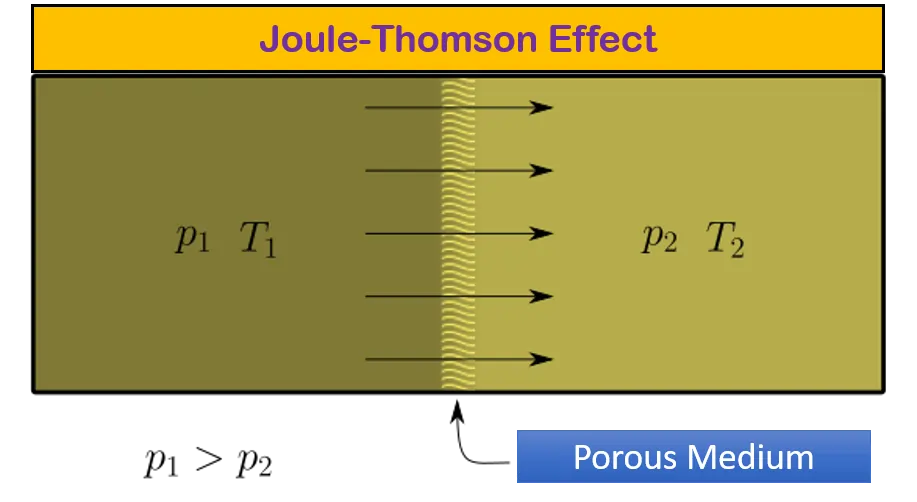
The mathematical formula for the Joule-Thomson effect involves the Joule-Thomson coefficient (\(\mu_{JT}\)), which represents the rate of change of temperature (\(T\)) with respect to pressure (\(P\)) at constant enthalpy (\(H\)). The formula is given by:

\[ \mu_{JT} = \left( \frac{\partial T}{\partial P} \right)_H \]

To express the temperature change (\(\Delta{T}\)) resulting from a pressure change(\(\Delta{P}\)) during a Joule-Thomson expansion, we use:

\[ \Delta T = \mu_{JT} \Delta P \]

where,

• \(\mu_{JT}\) is the Joule-Thomson coefficient, measured in Kelvin per Pascal (K/Pa)
• \(H\) is the enthalpy
• \(\Delta T\) is the change in temperature, measured in Kelvin (K)
• \(\Delta P\) is the change in pressure, measured in Pascal (Pa)

Related: Other Heat Transfer Calculators

Joule-Thomson Coefficient (\(\mu_{JT}\)) Calculation

The equation for \(\mu_{JT}\) can be derived from this equation by applying the Maxwell relations and the definition of specific heat at constant pressure \(C_P\). This equation is derived from the Van der Waals equation of state for real gases. The final equation is:

\[ \mu_{JT} = \frac{1}{C_P} \left( \frac{2a}{RT} – b \right) \]

where,

• \(\mu_{JT}\) is measured in K/Pa
• \(C_P\) is measured in J/(mol.K)
• a and b are measured in (Pa.m⁶)/(mol²) and m³/mol respectively

Above equation shows that the Joule-Thomson coefficient depends on the temperature \(T\), the specific heat at constant pressure \(C_P\), and the Van der Waals constants (\(a\) and \(b\)).

The term \(\frac{2a}{RT}\) represents the intermolecular attractive forces, and \(b\) represents the volume occupied by the gas molecules. The ratio \(\frac{1}{C_P}\) scales these effects by the gas’s capacity to store heat.

Note: Above equation is the simplified model and may not accurately predict the behavior of real gases under all conditions. It is most accurate for gases near their boiling point and at low pressures.

Related: Kirchoff’s Law of Thermal Radiation, Wien’s Displacement Law

Joule-Thomson Coefficient (\(\mu_{JT}\)) Calculator

This calculator computes the Joule-Thomson coefficient \(\mu{JT}\), that describes the change in temperature of a real gas when it is allowed to expand or compress at constant enthalpy.

To calculate this coefficient, the user inputs the temperature (T), the specific heat capacity at constant pressure \(C_P\), and the Van der Waals constants ‘a’ and ‘b’, which account for the intermolecular forces and finite size of gas molecules, respectively.

Note: User can input the values of a, b and \(C_P\) from the table given below this page.

Source: For \(C_P\) values – Table of Heat Capacity values

Source: For vander walls a and b constants – Vander walls constants

Substance	a (Pa. m6/mol2)	b (m3/mol)	CP (J/mol.K)
Argon	0.1355	0.00003201	20.7862
Carbon dioxide	0.364	0.00004267	36.94
Ethanol	1.218	0.00008407	112
Helium	0.00346	0.0000238	20.7862
Hydrogen	0.02476	0.00002661	28.82
Hydrogen sulfide	0.449	0.00004287	34.6
Mercury	0.82	0.00001696	27.98
Neon	0.02135	0.00001709	20.7862
Nitrogen	0.137	0.0000387	29.12
Oxygen	0.1382	0.00003186	29.38
Water	0.5536	0.00003049	75.34

Joule- Thomson Effect – Inversion Temperature

The Inversion Temperature is a characteristic temperature below which a gas expands adiabatically into a region of low pressure through a porous plug with a fall in temperature. It is the temperature at which the Joule-Thomson coefficient (µ_JT) is zero. This means that the gas does not cool (µ_JT > 0) or warm (µ_JT < 0) when it experiences expansion.

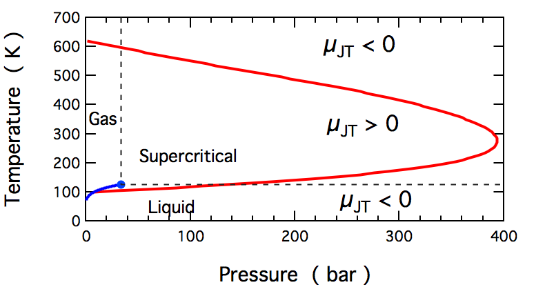
Image source: Wikipedia – Inversion Temperature

Derivation of Joule-Thomson Coefficient

The first step in obtaining Joule–Thomson coefficient involves the three variables 𝑇, 𝑃, and 𝐻. A useful result can be obtained by applying the cyclic rule; in terms of these three variables that rule may be written as

\(\left(\frac{\partial T}{\partial P}\right)_H \left(\frac{\partial H}{\partial T}\right)_P \left(\frac{\partial P}{\partial H}\right)_T = -1\)

Each of the three partial derivatives in this expression has a specific meaning. The first is \(\mu_{JT}\)​, the Joule–Thomson coefficient, the second is the constant pressure heat capacity, \(C_P\)​, defined by

\(C_P = \left(\frac{\partial P}{\partial T}\right)_H\)

​and the third is the inverse of the isothermal Joule–Thomson coefficient, μ_T​, defined by

\(\mu_T = \left(\frac{\partial P}{\partial H}\right)_T\)

This last quantity is more easily measured than 𝜇_JT​. Thus, the expression from the cyclic rule becomes

\(\mu_{JT} = -\frac{\mu_T}{C_P}\)

This equation can be used to obtain Joule–Thomson coefficients from the more easily measured isothermal Joule–Thomson coefficient. It is used in the following to obtain a mathematical expression for the Joule–Thomson coefficient in terms of the volumetric properties of a fluid.

To proceed further, the starting point is the fundamental equation of thermodynamics in terms of enthalpy; this is

\(𝑑𝐻=𝑇𝑑𝑆+𝑉𝑑𝑃\)

Now “dividing through” by 𝑑𝑃, while holding temperature constant, yields

\(\left(\frac{\partial H}{\partial P}\right)_T = T \left(\frac{\partial S}{\partial P}\right)_T + V\)

The partial derivative on the left is the isothermal Joule–Thomson coefficient, 𝜇_𝑇​, and the one on the right can be expressed in terms of the coefficient of thermal expansion via a Maxwell relation. The appropriate relation is

\(\left(\frac{\partial P}{\partial S}\right)_T = -\left(\frac{\partial V}{\partial T}\right)_P = -V\alpha\)

where 𝛼 is the cubic coefficient of thermal expansion. Replacing these two partial derivatives yields

\(\mu_T = -TV\alpha + V\)

This expression can now replace 𝜇_𝑇 in the earlier equation for 𝜇_JT​ to obtain:

\(\mu_{JT} \equiv \left(\frac{\partial P}{\partial T}\right)_H \)

\(\mu_{JT} = \frac {V}{C_P} (\alpha T – 1)\)

This provides an expression for the Joule–Thomson coefficient in terms of the commonly available properties heat capacity, molar volume, and thermal expansion coefficient.

It shows that the Joule–Thomson inversion temperature, at which 𝜇_JT​ is zero, occurs when the coefficient of thermal expansion is equal to the inverse of the temperature. Since this is true at all temperatures for ideal gases (see expansion in gases), the Joule–Thomson coefficient of an ideal gas is zero at all temperatures.

Python code for Joule-Thomson Coefficient

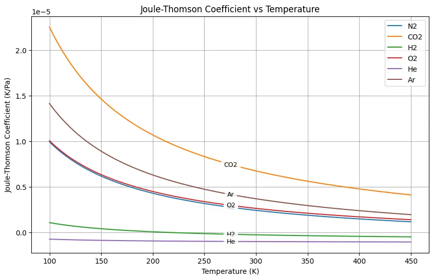
This python code helps user to plot the Joule–Thomson coefficient \(\mu{JT}\) as a function of temperature for various real gases, like Nitrogen, Carbon Dioxide, Hydrogen, Oxygen, Helium, and Argon. The Joule–Thomson coefficient indicates the temperature change of a gas during a throttling process at constant enthalpy.

Note: This Python code solves the specified problem. Users can copy the code and run it in a suitable Python environment. By adjusting the input parameters, users can observe how the output changes accordingly.

import numpy as np
import matplotlib.pyplot as plt

# Constants
R = 8.314  # Gas constant in J/(mol*K)

# Specific heat capacities at constant pressure (Cp) in J/(mol*K)
Cp_values = {
    'N2': 29.124,  # Nitrogen
    'CO2': 36.94,  # Carbon dioxide
    'H2': 28.836,   # Hydrogen
    'O2': 29.376,   # Oxygen
    'He': 20.786,   # Helium
    'Ar': 20.7862,   # Argon
}

# Van der Waals parameters: a and b
# Values are in (Pa*m^6)/(mol^2) for 'a' and in m^3/mol for 'b'
van_der_waals_parameters = {
    'N2': {'a': 1.365e-1, 'b': 3.91e-5},
    'CO2': {'a': 3.640e-1, 'b': 4.28e-5},
    'H2': {'a': 2.405e-2, 'b': 2.71e-5},
    'O2': {'a': 1.360e-1, 'b': 3.18e-5},
    'He': {'a': 3.46e-3, 'b': 2.38e-5},
    'Ar': {'a': 1.355e-1, 'b': 3.20e-5},
}

# Temperature range for plotting (in Kelvin)
T = np.linspace(100, 450, 300)

# Function to calculate Joule-Thomson coefficient
def joule_thomson_coefficient(gas, T):
    a = van_der_waals_parameters[gas]['a']
    b = van_der_waals_parameters[gas]['b']
    Cp = Cp_values[gas]
    mu_JT = (1 / Cp) * ((2 * a) / (R * T) - b)
    return mu_JT

# Plotting
plt.figure(figsize=(10, 6))
for gas in Cp_values.keys():
    mu_JT = joule_thomson_coefficient(gas, T)
    plt.plot(T, mu_JT, label=gas)
    # Find a point to place the label
    label_x = T[len(T) // 2]
    label_y = mu_JT[len(T) // 2]
    plt.text(label_x, label_y, gas, fontsize=9, ha='center', va='center', 
             bbox=dict(facecolor='white', alpha=0.8, edgecolor='none'))

plt.title('Joule-Thomson Coefficient vs Temperature')
plt.xlabel('Temperature (K)')
plt.ylabel('Joule-Thomson Coefficient (K/Pa)')
plt.legend()
plt.grid(True)
plt.show()

Output:

Resources

• “Thermodynamics: An Engineering Approach” by Yunus A. Çengel and Michael A. Boles
• “Introduction to Chemical Engineering Thermodynamics” by J.M. Smith, H.C. Van Ness, and M.M. Abbott
• NPTEL Lectures on Thermodynamics
• Research Paper: A Joule-Thomson apparatus for the determination of the enthalpies of gases
• THE JOULE-THOMSON EXPERIMENT

Disclaimer: The Solver provided here is for educational purposes. While efforts ensure accuracy, results may not always reflect real-world scenarios. Verify results with other sources and consult professionals for critical applications. Contact us for any suggestions or corrections.