Table of Contents
Heat Transfer through Convection – Theory
Convective heat transfer is a process in which heat is transferred between a solid surface and a fluid (liquid or gas) in motion. It occurs due to the combined effects of conduction and fluid motion. The movement of fluid transfers heat from hotter regions to cooler regions.
The rate of heat transfer through convection can be calculated using Newton’s Law of Cooling/Heating, which states:
𝑄 = ℎ 𝐴 Δ𝑇
Where:
- 𝑄 is the rate of heat transfer (in watts or BTUs per second),
- ℎ is the convective heat transfer coefficient (in watts per square meter per degree Celsius or BTUs per square foot per hour per degree Fahrenheit),
- 𝐴 is the surface area through which heat is being transferred (in square meters or square feet), and
- Δ𝑇 is the temperature difference between the surface and the surrounding fluid (in degrees Celsius or degrees Fahrenheit).\
Related: Inverse Square Law for Radiation
Convective Heat Transfer Calculator
This tool is designed for engineers and researchers to predict and analyze heat transfer between surfaces and fluids in motion i.e heat transfer through convection. Rate of heat transfer can be calculated by inputting parameters like surface Area, Temperature difference and heat transfer coefficients.
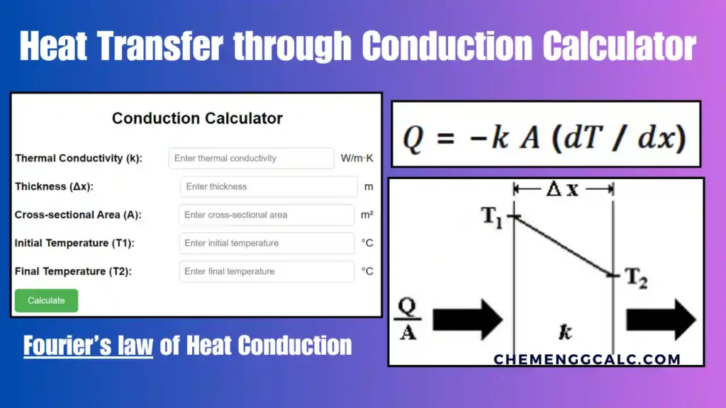
Related: Heat Transfer through Conduction Calculator
Related: Bernoulli’s Equation Calculator / Solver
Convective heat transfer is crucial in various engineering and scientific applications, such as cooling systems, HVAC (Heating, Ventilation, and Air Conditioning), and thermal management in industries.
Types of Convective Heat Transfer
Convection is classified into two main types: Natural Convection and Forced Convection.
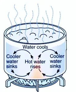
Natural Convection occurs when the motion of the fluid is caused by density differences within the fluid itself. Natural convection is often observed in various everyday situations, such as the rising of warm air near a heat source, the circulation of water in a pot heated on a stove, and the movement of air in a room heated by a radiator.
Forced Convection occurs when the motion of the fluid is induced by external means, such as fans, pumps, or blowers. In forced convection, an external force is applied to the fluid to enhance its motion and heat transfer. For example, Air circulation inside a room due to the operation of a fan, or the flow of coolant through the tubes of a heat exchanger driven by a pump.
Key differences between Natural Convection and Forced Convection
| Natural Convection | Forced Convection |
|---|---|
| Natural convection is driven by buoyancy forces resulting from temperature differences | Forced convection is driven by external mechanical means |
| Fluid motion arises spontaneously due to density variations | Fluid motion is induced by external devices |
| Natural convection is common in many natural and domestic scenarios | Forced convection is prevalent in engineered systems where precise control over heat transfer rates is required |
Example Problem on Convective Heat Transfer
What is the bulk temperature of the environment (\(T_b\)) if a flat wall, covered with a 1-inch thick layer of insulation (with a thermal conductivity of \(0.8 \, \text{Btu/hr-ft-°F}\)), has an inner wall temperature of \(600°F\) and loses heat to the environment by convection on the surface of the insulation? The average value of the convection heat transfer coefficient on the insulation surface is \(950 \, \text{Btu/hr-ft²-°F}\), and the outer surface of the insulation must not exceed \(105°F\).
Solution:
First, let’s find the heat flux (\(Q˙′′\)) through the insulation using the formula:
\[Q˙ = kA\left(\frac{ΔT}{Δx}\right)\]
\[Q˙ = (0.8 \, \text{Btu/hr-ft-°F}) \times \left(\frac{600°F – 105°F}{\frac{1}{12} \, \text{ft}}\right)\]
\[Q˙ = 4752 \, \text{Btu/hr-ft²}\]
Next, we can find the bulk temperature of the environment (\(T_b\)) using the formula for convection heat transfer:
\[Q˙ = hA(T_{\text{ins}} – T_b)\] \[T_b = T_{\text{ins}} – \frac{Q˙}{hA}\]
\[T_b = 105°F – \frac{4752 \, \text{Btu/hr-ft²}}{950 \, \text{Btu/hr-ft²-°F} \times 100 \, \text{ft}²}\] \[T_b ≈ 100°F\]
Thus, the bulk temperature of the environment is approximately \(100°F\).
Derivation for Newton’s Law of Cooling
Let’s start with Newton’s Law of Cooling: The rate of change of temperature with respect to time \(( \frac{dT}{dt} )\) is proportional to the temperature difference between the object \(( T )\) and the surrounding medium \(( T_S )\). This can be expressed as: \[ \frac{dT}{dt} = k(T – T_S) \] where \( k \) is the proportionality constant. Let \( T_f \) be the temperature at time \( t \) and \( T_0 \) be the initial temperature.
Integrating both sides:
\[ \int_{T_0}^{T_f} \frac{dT}{T-T_S} = -\int_{0}^{t} k \, dt \]
\[ \ln|T_f – T_S| – \ln|T_0 – T_S| = -k \cdot t \]
\[ \ln\left(\frac{T_f – T_S}{T_0 – T_S}\right) = -k \cdot t \]
\[ \frac{T_f – T_S}{T_0 – T_S} = e^{-k \cdot t} \]
\[ T_f – T_S = (T_0 – T_S) \cdot e^{-k \cdot t} \]
\[ T_f = T_S + (T_0 – T_S) \cdot e^{-k \cdot t} \]
This is the formula for Newton’s Law of Cooling: \[ T(t) = T_S + (T_0 – T_S) \cdot e^{-k \cdot t} \] This equation describes how the temperature of an object changes over time as it loses heat to its surroundings through convection. \( T(t) \) is the temperature of the object at time \( t \), \( T_S \) is the surrounding temperature, \( T_0 \) is the initial temperature of the object, and \( k \) is the constant of proportionality.
Python Code for Newton’s Law of Cooling – Time vs Temperature
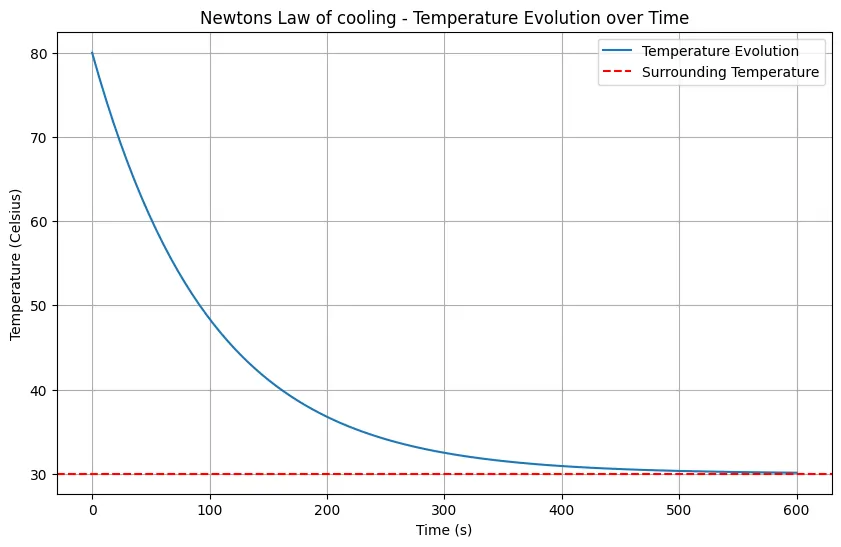
This Python code enables users to explore heat transfer through convection using Newton’s law of cooling. By adjusting parameters like initial and surrounding temperatures, heat transfer coefficient, object surface area, and simulation duration, users can observe how an object’s temperature changes over time.
Note: This Python code solves the specified problem. Users can copy the code and run it in a suitable Python environment. By adjusting the input parameters, users can observe how the output changes accordingly.
import numpy as np
import matplotlib.pyplot as plt

def newtons_law_of_cooling(T_initial, T_surrounding, k, A, t):
    """
    Solve Newton's law of cooling for temperature over time.

    Args:
    - T_initial: Initial temperature of the object (in Celsius)
    - T_surrounding: Temperature of the surrounding environment (in Celsius)
    - k: Heat transfer coefficient (in W/m^2*K)
    - A: Surface area of the object (in m^2)
    - t: Time (in seconds)

    Returns:
    - T: Temperature of the object at time t (in Celsius)
    """
    T = T_surrounding + (T_initial - T_surrounding) * np.exp(-k * A * t)
    return T

def plot_temperature_evolution(T_initial, T_surrounding, k, A, t_end, num_points=100):
    """
    Plot the evolution of temperature over time using Newton's law of cooling.

    Args:
    - T_initial: Initial temperature of the object (in Celsius)
    - T_surrounding: Temperature of the surrounding environment (in Celsius)
    - k: Heat transfer coefficient (in W/m^2*K)
    - A: Surface area of the object (in m^2)
    - t_end: End time (in seconds)
    - num_points: Number of points to plot

    Returns:
    - None (plots the graph)
    """
    t_values = np.linspace(0, t_end, num_points)
    T_values = newtons_law_of_cooling(T_initial, T_surrounding, k, A, t_values)

    plt.figure(figsize=(10, 6))
    plt.plot(t_values, T_values, label='Temperature Evolution')
    plt.axhline(y=T_surrounding, color='r', linestyle='--', label='Surrounding Temperature')
    plt.title('Newtons Law of cooling - Temperature Evolution over Time')
    plt.xlabel('Time (s)')
    plt.ylabel('Temperature (Celsius)')
    plt.legend()
    plt.grid(True)
    plt.show()

# Parameters
T_initial = 80  # Initial temperature of the object (in Celsius)
T_surrounding = 30  # Temperature of the surrounding environment (in Celsius)
k = 0.1  # Heat transfer coefficient (in W/m^2*K)
A = 0.10  # Surface area of the object (in m^2)
t_end = 600  # End time (in seconds)

# Plot temperature evolution
plot_temperature_evolution(T_initial, T_surrounding, k, A, t_end)
Output:
Resources:
- “Fundamentals of Heat and Mass Transfer” by Theodore L. Bergman, Adrienne S. Lavine, Frank P. Incropera, and David P. DeWitt.
- “Introduction to Heat Transfer” by Theodore L. Bergman, Adrienne S. Lavine, Frank P. Incropera, and David P. DeWitt.
- “Convective Heat and Mass Transfer” by S. Mostafa Ghiaasiaan.
- “Heat and Mass Transfer: Fundamentals and Applications” by Yunus A. Cengel and Afshin J. Ghajar.
- https://github.com/FluidityProject/fluidity
Disclaimer: The Solver provided here is for educational purposes. While efforts ensure accuracy, results may not always reflect real-world scenarios. Verify results with other sources and consult professionals for critical applications. Contact us for any suggestions or corrections.

