Table of Contents
Cooling time of a sphere is an important concept in many heat transfer applications where thermal management is needed. Spheres are commonly used shapes in industrial applications due to their optimal surface-to-volume ratio, minimizing material usage while maximizing heat exchange. It is the case which often seen in areas such as metallurgy, chemical engineering, and environmental controls.
Cooling Time of a Sphere
The cooling time of a sphere is the time taken for the object to cool from an initial temperature to a desired final temperature when exposed to a surrounding fluid at a constant ambient temperature.
The cooling process is followed by convective heat transfer, where heat is transferred from the surface of the sphere to the surrounding environment. The cooling time can be calculated using the lumped capacitance method, which assumes that the temperature within the sphere is uniform at any given time.
The cooling time of a sphere is given by the equation:
\[t = \frac{\rho c_p V}{h A} \ln \left( \frac{T_i – T_\infty}{T_f – T_\infty} \right)\]
or
\[t = \tau \ln \left( \frac{T_i – T_\infty}{T_f – T_\infty} \right)\]
where in S.I. units,
- t is the cooling time (s)
- \(\tau = \frac{\rho c_p V}{h A} \) is the thermal time constant (s)
- ρ is the density of the sphere material (kg/m³)
- cp is specific heat capacity (J/kg·K)
- V is volume of the sphere (m³)
- h is convective heat transfer coefficient (W/m²·K)
- A is the surface area of the sphere (m²)
- Ti is the initial temperature of the sphere (K or °C)
- Tf is the final temperature of the sphere (K or °C)
- T∞ ambient temperature (K or °C)
Related: Heat Transfer through Conduction Calculator – Fourier’s law
Related: Hydraulic Diameter Calculator for Circular and Non-Circular cross-section
Cooling Time of a Sphere Calculator
This Cooling Time of a Sphere Calculator helps user to determine the cooling time of a spherical object using the lumped capacitance method. Based on user choice i.e cooling time, final temperature, or initial temperature can be calculated by inputting the values.
Related: Heat Transfer through Convection Calculator – Newton’s Law of Cooling
Related: Joule-Thomson Effect – Coefficient Calculation for CO2 and N2
What is the Lumped Capacitance Method?
The lumped capacitance method is an easy approach to study transient heat transfer (unsteady state), where temperature changes over time are considered. This method assumes that the temperature within an object (sphere) is uniform at any given moment.
- In Lumped system analysis internal thermal gradients are negligible, and the object cools uniformly. This makes the equation easier to handle instead of solving the complex partial differential equations of transient heat conduction.
- For the lumped capacitance method to be valid, the Biot number (Bi) must be less than 0.1. If the Biot number is larger, more complex methods that account for internal temperature gradients are needed.
Related: Biot Number Calculator – Significance and Calculations
Related: Critical Thickness of Insulation Calculator for Cylinder and Sphere
Derivation for Convection Cooling Time of a Sphere
For the derivation for cooling time of a sphere we will assume the lumped capacitance method and heat loss occurs due to convection between the surface of the sphere and the surrounding fluid at temperature T∞. Also the Biot number (Bi=hLc/k) is less than 0.1 to validate the assumption.
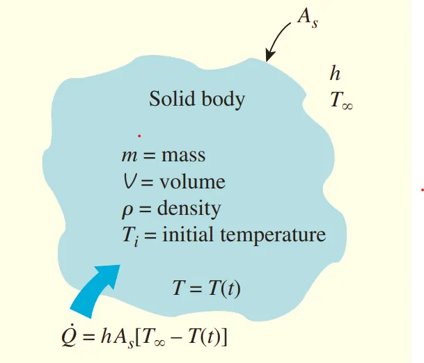
Consider a solid body with of mass m, volume V, surface area As, density ρ, and specific heat cp initially at a uniform temperature Ti as shown in figure.
At time t, the body is at temperature T and heat transfer take place from body to its environment at temperature T∞ with heat transfer coefficient h.
According to principle of energy conservation Heat transfer into the body during dt is equal to the increase in the
energy of the body during dt.
During a differential time interval dt, the temperature of the body rises by a differential amount dT and is given as:
\[h A_s (T_\infty – T) dt = m c_p dT\]
Since the mass m can be expressed as \(m = \rho V\), therefore, above equation can be rewritten as
\[h A_s (T_\infty – T) dt = \rho V c_p dT\]
where:
- dt is the differential time interval (s)
- dT is the differential temperature change of the body (K or °C)
- ρ is the density of the sphere material (kg/m³)
- cp is specific heat capacity (J/kg·K)
- V is volume of the sphere (m³)
- h is convective heat transfer coefficient (W/m²·K)
- A is the surface area of the sphere (m²)
- Ti is the initial temperature of the sphere (K or °C)
- T∞ ambient temperature (K or °C)
Now, rearranging the equation to separate the variables T and t:
\[\frac{dT}{T – T_\infty} = – \frac{h A_s}{\rho V c_p} dt\]
Integrating both side with limits from the initial temperature Ti to the temperature T(t) at any time t
\[\int_{T_i}^{T(t)} \frac{dT}{T – T_\infty} = – \int_0^t \frac{h A_s}{\rho V c_p} dt\]
\[\ln \left( \frac{T(t) – T_\infty}{T_i – T_\infty} \right) = – \frac{h A_s}{\rho V c_p} t\]
taking exponent both side we get:
\[\frac{T(t) – T_\infty}{T_i – T_\infty} = e^{-\frac{h A_s}{\rho V c_p} t}\]
rearranging above equation to get,
\[T(t) = T_\infty + (T_i – T_\infty) e^{-\frac{h A_s}{\rho V c_p} t}\]
Also Read: Antoine Equation Calculator for Vapour Pressure versus Temperature Calculations
Also Read: Clausius Clapeyron Equation Calculator, Derivation and Applications
Example Problem on Cooling Time of a Sphere
The temperature of a gas stream is to be measured by a thermocouple whose junction can be approximated as a 1-mm-diameter sphere. The properties of the junction are k = 35 W/m·K, ρ = 8500 kg/m3, and cp = 320 J/kg·K, and the convection heat transfer coefficient between the junction and the gas is h = 210 W/m2·K. Determine how long it will take for the thermocouple to read 99 percent of the initial temperature difference.
To find the time required for the thermocouple to read 99% of the initial temperature difference between the thermocouple junction and the gas. Using equation:
\[\frac{T(t) – T_\infty}{T_i – T_\infty} = e^{-\frac{t}{\tau}}\]
For the thermocouple to reach 99% of the initial temperature difference means that:
\[\frac{T(t) – T_\infty}{T_i – T_\infty} = 0.01\]
Substituting this into the equation:
\[0.01 = e^{-\frac{t}{\tau}}\]
Taking the natural logarithm of both sides:
\[\ln(0.01) = -\frac{t}{\tau}\]
\[t = \frac{\ln(0.01)}{-\frac{1}{\tau}}\]
we know that, \(\tau = \frac{\rho c_p L_c}{h}\) here \(L_c = \frac{r}{3}\) for sphere, now substituting the values into the formula for \(\tau\)
\[\tau = \frac{\rho c_p L_c}{h} = \frac{(8500)(320)(1.67 \times 10^{-4} )}{210}\]
\[\tau = 2.164 \, \text{seconds}\]
now, putting the value of \(\tau = 2.164\) into the equation for t, we get
\[t = \frac{\ln(0.01)}{-\frac{1}{2.164}}\]
\[t = \frac{-4.605}{-\frac{1}{2.164}} = 9.96 \, \text{seconds}\]
It will take approximately 10 seconds for the thermocouple to read 99% of the initial temperature difference between the thermocouple junction and the gas.
Also Read: Van der Waals Equation Calculator and PV Isotherm for Real Gases
Python Code for cooling Time calculation
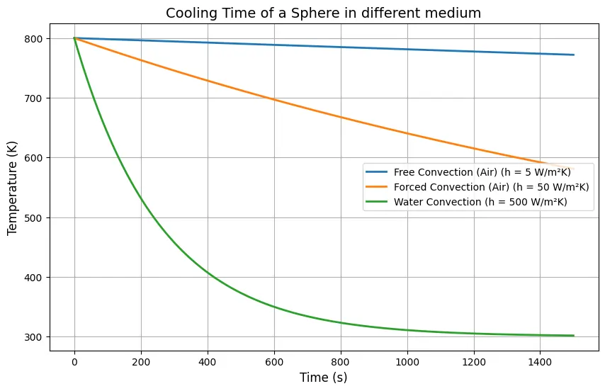
This Python code simulates and plots the cooling time of a sphere different convective heat transfer coefficients (h). The code calculates the temperature of the sphere over time and plots the cooling profiles, showing how the sphere cools faster in environments with higher h, such as water, compared to air.
Note: This Python code solves the specified problem. Users can copy the code and run it in a suitable Python environment. By adjusting the input parameters, users can observe how the output changes accordingly.
import numpy as np
import matplotlib.pyplot as plt

# Constants
T_i = 800  # Initial temperature of the sphere (K)
T_inf = 300  # Ambient temperature (K)
r = 0.1  # Radius of the sphere (m)
rho = 7800  # Density of the material (kg/m^3), example: steel
c_p = 500  # Specific heat capacity (J/kg*K), example: steel

# Convective heat transfer coefficients for different environments
h_values = {
    "Free Convection (Air)": 5,
    "Forced Convection (Air)": 50,
    "Water Convection": 500
}

# Calculate surface area and volume of the sphere
A_s = 4 * np.pi * r**2  # Surface area of the sphere
V = (4/3) * np.pi * r**3  # Volume of the sphere

# Time array (seconds)
time = np.linspace(0, 1500, 500)  # Time from 0 to 2000 seconds

# Function to calculate temperature over time
def temperature_profile(time, T_i, T_inf, h, A_s, rho, V, c_p):
    T = T_inf + (T_i - T_inf) * np.exp(- (h * A_s / (rho * V * c_p)) * time)
    return T

# Plotting the temperature profiles for different h values
plt.figure(figsize=(10, 6))

for label, h in h_values.items():
    # Calculate temperature over time for each h value
    temperature = temperature_profile(time, T_i, T_inf, h, A_s, rho, V, c_p)
    plt.plot(time, temperature, label=f'{label} (h = {h} W/m²K)', linewidth=2)

# Plot formatting
plt.title('Cooling Time of a Sphere in different medium', fontsize=14)
plt.xlabel('Time (s)', fontsize=12)
plt.ylabel('Temperature (K)', fontsize=12)
plt.grid(True)
plt.legend(loc='right')
plt.show()
Output:
Resources
- Heat Transfer a Practical Approach – Book by Yunus A Çengel
- “Fundamentals of Heat and Mass Transfer” by Theodore L. Bergman, Adrienne S. Lavine, Frank P. Incropera, and David P. DeWitt.
- “Heat Transfer Book” by David W. Hahn.
- “Conduction of Heat in Solids” by H.S. Carslaw and J.C. Jaeger.
- “Introduction to Heat Transfer” by Frank P. Incropera, David P. DeWitt, Theodore L. Bergman, and Adrienne S. Lavine.
Disclaimer: The Solver provided here is for educational purposes. While efforts ensure accuracy, results may not always reflect real-world scenarios. Verify results with other sources and consult professionals for critical applications. Contact us for any suggestions or corrections

