Have you ever noticed how honey flows slowly compared to water? That’s because of a property of fluids called viscosity, which describes their resistance to flow. Newton’s law of viscosity describes the relationship between a fluid’s resistance to flow (viscosity) and the shear stress applied to it.
Table of Contents
Newton’s Law of Viscosity
Newton’s Law of Viscosity states that the shear stress \(\tau\) experienced by a fluid is directly proportional to the velocity gradient, or shear rate du/dy, within the fluid. Such fluids which obeys this law are known as Newtonian Fluids.
In mathematical terms, newton’s law of viscosity is expressed as:
\[ \tau =\frac{F}{A} = \mu \frac{du}{dy} \]
where,
- \(\tau\) is the shear stress (measured in units of force per unit area)
- \(\mu\) is the Dynamic viscosity of the fluid (measured in units of Pascal-seconds or poise)
- \(\frac{du}{dy}\) is the shear rate (represents the rate of change of velocity with respect to distance perpendicular to the direction of flow)
Related: Ergun Equation Calculator for Pressure Drop in Packed Bed Column
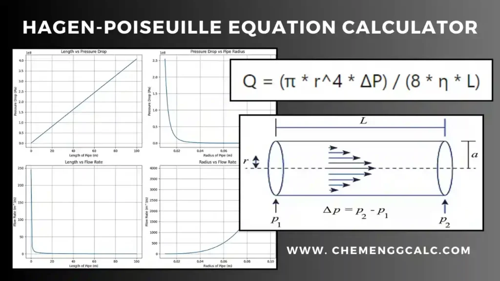
Related: Hagen-Poiseuille Equation Calculator / Poiseuille’s Law Solver
Newton’s Law of Viscosity Calculator
This calculator helps users calculate velocity gradient, viscosity, force, and area using Newton’s Law of Viscosity. Enter the needed values to calculate the chosen parameter, and the code will compute and show the result. It provides an easy-to-use interface for studying fluid dynamics.
Related: Friction Factor Calculator Moody’s Diagram for Smooth and Rough Pipes
Related: Head Loss or Pressure Loss Calculator using Darcy-Weisbach Equation
Terminologies Used in Newton’s Law of Viscosity
Shear stress
Imagine a fluid sandwiched between two plates. When one plate moves relative to the other, the fluid experiences a dragging force. This force per unit area acting parallel to the layers of the fluid is called shear stress.
Velocity gradient
As the plate moves, the fluid layers closer to it will move faster than the layers further away. This difference in velocity across the fluid is called the velocity gradient.

Assumption for Newton’s Law of Viscosity
- The fluid is assumed to be in a steady state with constant flow conditions
- Fluid being the homogeneous and isotropic, that means properties (such as viscosity) are uniform throughout and do not vary with direction
- No Slip Boundary Condition – The velocity at the boundary assumed to be zero
- This law is applicable to both laminar and turbulent flows, it’s often used for laminar flow conditions
Dynamic vs. Kinematic Viscosity
Dynamic viscosity reflects the internal friction a fluid experiences when external forces or stresses try to make it flow. Imagine honey – its high dynamic viscosity means it needs a strong force to overcome its internal friction and move easily. The SI unit for dynamic viscosity is Pascal-second (Pa·s), and it’s often represented by the symbol μ (mu).
Its formula relates shear stress (τ, tau) to the velocity gradient (du/dy) within the fluid: τ = μ * (du/dy).
Kinematic viscosity, focuses on a fluid’s internal resistance specifically under the influence of gravity. It essentially tells you how quickly a fluid can flow due to gravity acting on it. Think of how water flows much faster than oil – their kinematic viscosities differ significantly.
Kinematic viscosity \(v\) is calculated by dividing the dynamic viscosity \(\mu\) by the fluid’s density \(\rho\). This value is measured in square meters per second (m²/s).
\[v = \frac{\mu}{\rho}\]
Related: Reynolds Number Calculator for a Circular Pipe
Example Problem on Newton’s Law of Viscosity
An infinite plate is moved over a second plate on a layer of liquid as shown. For small gap width, d, we assume a linear velocity distribution in the liquid. The liquid viscosity is 0.65 centipoise and its specific gravity is 0.88. Given values, u = 0.3 m/s , distance across the plate (d) = 0.3mm Determine:
- (a) The absolute viscosity of the liquid, in lbf s/ft2.
- (b) The kinematic viscosity of the liquid, in m²/s.
- (c) The shear stress on the upper plate, in lbf/ft2.
- (d) The shear stress on the lower plate, in Pa.
- (e) The direction of each shear stress calculated in parts (c) and (d).
Given:
- Viscosity of liquid (\(\mu\)) = 0.65 centipoise
- Specific Gravity (\(SG\)) = 0.88
- velocity, \(u\) = 0.3 m/s
- distance across the plate, d = 0.3 mm = 0.0003 m
(a) The absolute viscosity of the liquid, in lbf s/ft2
converting centipoise into lbf s/ft2 , 1cp = 2.088 * 10-4 lbf s/ft2
\( \mu = 0.65 \, \text{centipoise} * 0.0000208854 \, \text{lbf s/ft}^2/\text{centipoise} \)
\(\mu = 1.36 * 10^{-5}\) \(\text{lbf s/ft}^2 \)
(b) The kinematic viscosity of the liquid, in m²/s.
First, we will calculate the density (\(\rho\)) of the liquid using the specific gravity (SG) and the density of water (\(ρ_w\))
\( \rho = \text{SG} * \rho_w = 0.88 * 62.4 \, \frac{lbf}{ft^3}\)
therefore, \(\rho = 54.912 \) \(\frac{lbf}{ft^3}\)
now, using formula Kinematic Viscosity = Dynamic Viscosity / Density
\( \nu = (\mu)/(\rho) = \frac{0.00043745 \, \text{lbf s/ft}^2}{54.912 \, \text{lbf/ft}^3}\)
\( \nu = 7.957 * 10^{-6} \, \text{ft}^2/\text{s} \) = \(7.39 * 10^{-7} \frac{m^2}{s}\)
(c) The shear stress on the upper plate, in lbf/ft2.
using the formula for newton’s law of viscosity, \( \tau = \mu \frac{du}{dy} \)
let’s first calculate the velocity gradient,
\(\frac{du}{dy} = \frac{0.3}{0.0003} s^{-1}\) = \(1000 s^{-1}\)
\(\tau_{upper} = 1.36 * 10^{-5} \text{lbf s/ft}^2 * 1000 s^{-1} \)
\(\tau_{upper} = 0.0136 \frac{lbf}{ft^2}\)
(d) The shear stress on the lower plate, in Pa.
by converting into Pascals, using conversion \(\frac{lbf}{ft^2}\ = 47.88 Pa\)
\(\tau_{lower} = 0.0136 * 47.88 = 0.651 Pa\)
(e) The direction of each shear stress calculated in parts (c) and (d).
The shear stress on the upper plate (part c) acts in the opposite direction i.e negative x direction to the motion of the upper plate, while the shear stress on the lower plate (part d) in the positive x direction acts in the same direction as the motion of the upper plate.
Python Code for Newton’s Law of Viscosity
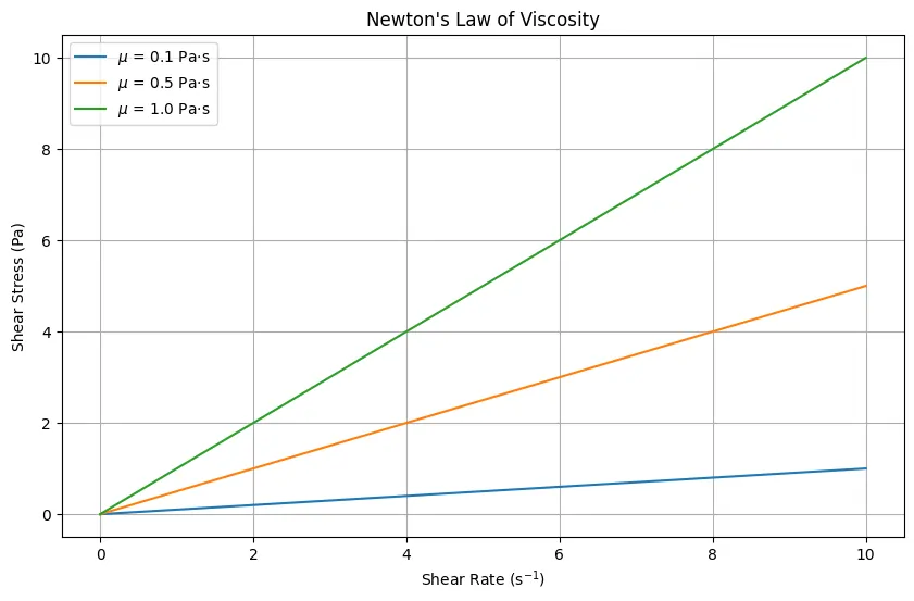
This python code calculates the shear stress \(\tau\) using Newton’s law of viscosity \( \tau =\mu \frac{du}{dy} \) for a range of shear rates \(\frac{du}{dy}\) at different \(\mu\) values. Then, it plots the relationship between shear stress and shear rate . Adjust the values of mu and du_dy as needed.
Note: This Python code solves the specified problem. Users can copy the code and run it in a suitable Python environment. By adjusting the input parameters, users can observe how the output changes accordingly.
import numpy as np
import matplotlib.pyplot as plt

# Constants
mu_values = [0.1, 0.5, 1.0]  # Dynamic viscosity (Pa·s) - Three different values
du_dy = np.linspace(0, 10, 100)  # Shear rate (s^-1)

# Plotting
plt.figure(figsize=(8, 6))

for mu in mu_values:
    # Calculate shear stress using Newton's law of viscosity
    tau = mu * du_dy

    # Plot shear stress vs. shear rate
    plt.plot(du_dy, tau, label=f'$\mu$ = {mu} Pa·s')

plt.xlabel('Shear Rate (s$^{-1}$)')
plt.ylabel('Shear Stress (Pa)')
plt.title("Newton's Law of Viscosity")
plt.grid(True)
plt.legend()
plt.show()
Output:
Resources:
- “Introduction to Fluid Mechanics and Fluid Machines” by Y. M. Joshi
- “Transport Phenomena” by Bird, Stewart, and Lightfoot.
- “Introduction to Chemical Engineering Fluid Mechanics” by William M. Deen.
- “Fluid Mechanics” by Frank M. White.
Disclaimer: The Solver provided here is for educational purposes. While efforts ensure accuracy, results may not always reflect real-world scenarios. Verify results with other sources and consult professionals for critical applications. Contact us for any suggestions or corrections.