Table of Contents
What is Bernoulli’s Equation and its Significance
Bernoulli’s equation or Bernoulli’s principle is a fundamental principle in fluid dynamics that relates the pressure, velocity, and elevation of a fluid flowing in a steady, incompressible manner. It’s named after the Swiss mathematician Daniel Bernoulli, who formulated it in the 18th century.
Bernoulli’s equation is significant because it describes the conservation of energy in a fluid flow system, illustrating how the different forms of energy—pressure energy, kinetic energy, and gravitational potential energy—are related and exchanged within the fluid.
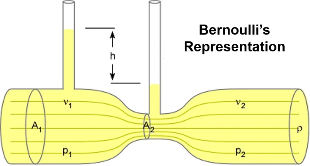
In its mathematical form, Bernoulli’s equation can be expressed as:
P + 1/2 ρv2 + ρgh = constant
Where:
- P is the pressure of the fluid at a certain point,
- ρ is the density of the fluid,
- v is the velocity of the fluid at that point,
- 𝑔 is the acceleration due to gravity,
- ℎ is the elevation of the point above a reference level,
- and the sum of these terms remains constant along any streamline of the flow.
This equation states that in a steady flow of an incompressible fluid, the sum of the pressure energy, kinetic energy, and potential energy per unit volume remains constant along any streamline.
Related: Hagen-Poiseuille Equation Calculator
Related: Other Fluid Mechanics Calculator
Assumptions and Limitations for Bernoulli’s Principle
- The fluid is incompressible, meaning its density remains constant regardless of changes in pressure or temperature.
- The fluid flow is steady, meaning that the velocity, pressure, and other flow properties do not change with time.
- The total mechanical energy per unit mass of the fluid remains constant along the streamline.
- The friction by viscous forces must be negligible.
Bernoulli’s Equation Calculator
This calculator simplifies the application of Bernoulli’s principle by computing pressure drops, energy losses, and velocity changes in fluid systems.
Related: Hydraulic Diameter Calculator for Circular and Non-Circular cross-section
Related: Reynolds Number Calculator for a Circular Pipe
Bernoulli’s equation has applications in various fields such as engineering, aerodynamics, and hydraulics.
- In engineering, it’s used to analyze and design systems involving fluid flow, such as pipelines, pumps, and turbines.
- In aerodynamics, it helps understand the principles of lift and drag on aircraft wings.
- In hydraulics, it’s used to design channels, dams, and water distribution systems.
Edition: Revised 2nd Edition, By: R. Byron Bird, Warren E. Stewart, Edwin N. Lightfoot
Comprehensive coverage of transport phenomena, including momentum, heat, and mass transfer. Updated content for better clarity.
Buy on AmazonExample Problem on Bernoulli’s Principle
Water is flowing in a fire hose with a velocity of 1.0 m/s and a pressure of 200000 Pa. At the nozzle the pressure decreases to atmospheric pressure (101300 Pa), there is no change in height. Use the Bernoulli equation to calculate the velocity of the water exiting the nozzle. (Hint: The density of water is 1000 kg/m3 and gravity g is 9.8 m/s2.
Given:
- v₁ = 1.0 m/s (water velocity in the hose)
- P₁ = 200,000 Pa (pressure in the hose)
- P₂ = 101,300 Pa (atmospheric pressure)
- ρ = 1000 kg/m³ (water density)
- g = 9.8 m/s² (acceleration due to gravity)
Applying Bernoulli’s equation (assuming constant height)
½ρv₁² + P₁ = ½ρv₂² + P₂solve for v2
v₂² = (2(P₁ - P₂) / ρ) + v₁²
v₂ = sqrt((2(P₁ - P₂) / ρ) + v₁²)
Substitute known values and calculate
v₂ = sqrt((2(200,000 Pa - 101,300 Pa) / 1000 kg/m³) + (1.0 m/s)²)
v₂ ≈ 14.05 m/s (round to two decimal places)
The calculated velocity of the water exiting the nozzle is approximately 14.05 m/s.
Python Code for solving Bernoulli’s Equation
This Python code helps you to learn the Bernoulli’s principle to analyze the relationship between fluid flow characteristics and energy distribution. This code generate subplots that shows how pressure energy, potential energy , and kinetic energy are changing with alterations in fluid height and velocity.
Note: This Python code solves the specified problem. Users can copy the code and run it in a suitable Python environment. By adjusting the input parameters, users can observe how the output changes accordingly.
"""# Explore the relationship between fluid flow characteristics and energy distribution.
# How do changes in fluid height and velocity affect pressure, potential, and kinetic energies?"""

import numpy as np
import matplotlib.pyplot as plt

# Constants
density = 1000  # Density of the fluid (kg/m^3)
gravity = 9.81  # Acceleration due to gravity (m/s^2)

# Function to calculate pressure energy
def pressure_energy(pressure):
    return pressure / (density * gravity)

# Function to calculate potential energy
def potential_energy(height):
    return density * gravity * height

# Function to calculate kinetic energy
def kinetic_energy(velocity):
    return 0.5 * density * velocity ** 2

# Heights to consider (m)
heights = np.linspace(0, 20, 100)

# Pressure (Pa), velocity (m/s) at each height
pressure = 100000  # pressure values in kPa
velocity = 5  # velocity values in m/s

# Create velocities to consider (m/s)
velocities = np.linspace(10, 30, 100)

# Initialize subplots
fig, (ax1, ax2) = plt.subplots(2, 1, figsize=(10, 8))

# Plotting for height changes
ax1.set_title("Energies vs. Height")
ax1.set_xlabel("Height (m)")
ax1.set_ylabel("Energy (J)")

# Calculate energies at each height
pressure_energies = pressure_energy(pressure) - density * gravity * heights
potential_energies = potential_energy(heights)
kinetic_energies = kinetic_energy(velocity)  # Using constant velocity for this plot

ax1.plot(heights, pressure_energies, label='Pressure Energy')
ax1.plot(heights, potential_energies, label='Potential Energy')
ax1.axhline(y=kinetic_energies, color='r', linestyle='--', label='Kinetic Energy')

ax1.legend()
ax1.grid(True)

# Plotting for velocity changes
ax2.set_title("Energies vs. Velocity")
ax2.set_xlabel("Velocity (m/s)")
ax2.set_ylabel("Energy (J)")

# Calculate energies at each velocity
pressure_energies = pressure_energy(pressure)
potential_energies = potential_energy(10)  # Using constant height for this plot
kinetic_energies = kinetic_energy(velocities)

ax2.plot(velocities, pressure_energies * np.ones_like(velocities), label='Pressure Energy')
ax2.plot(velocities, potential_energies * np.ones_like(velocities), label='Potential Energy')
ax2.plot(velocities, kinetic_energies, label='Kinetic Energy')

ax2.legend()
ax2.grid(True)

plt.tight_layout()
plt.show()
Output:
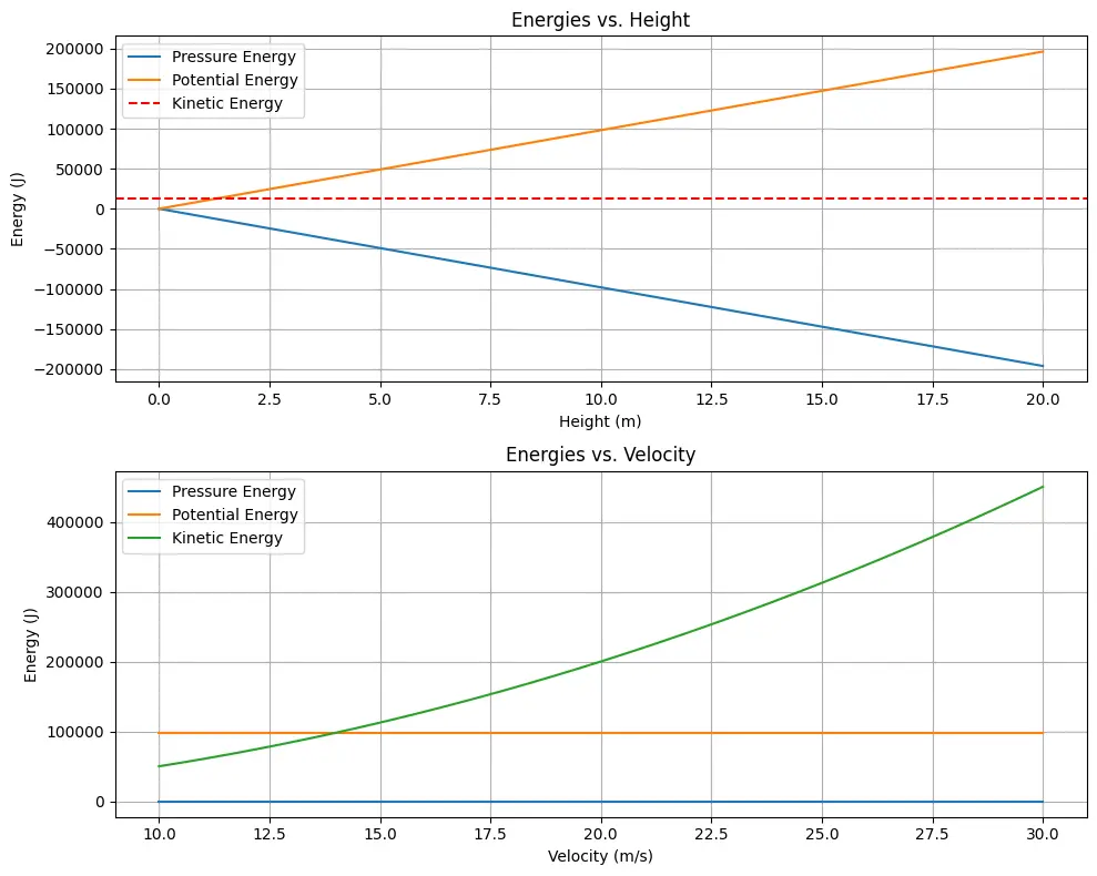
Python Code:
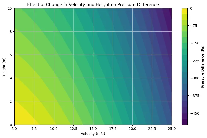
This code visualizes the effect of changes in velocity and height on the pressure difference according to Bernoulli’s principle. It calculates the pressure differences for a range of velocities and heights using Bernoulli’s equation and then plots a contour plot to illustrate how the pressure difference varies with changes in both velocity and height.
import numpy as np
import matplotlib.pyplot as plt

# Constants
density = 1.225  # Density of air in kg/m^3
velocity_range = np.linspace(5, 25, 100)  # Range of velocities (m/s)
height_range = np.linspace(0, 10, 100)     # Range of heights (m)

# Function to calculate pressure using Bernoulli's principle
def calculate_pressure(velocity, height):
    constant = 0.5 * density * velocity_range[0]**2 + density * 9.81 * height_range[0]  # Calculate constant for minimum velocity and height
    return constant - (0.5 * density * velocity**2 + density * 9.81 * height)  # Using Bernoulli's equation

# Calculate pressure differences for varying velocities and heights
pressure_differences = np.zeros((len(velocity_range), len(height_range)))
for i, velocity in enumerate(velocity_range):
    for j, height in enumerate(height_range):
        pressure_differences[i, j] = calculate_pressure(velocity, height)

# Plotting
plt.figure(figsize=(10, 6))

# Create a contour plot for pressure differences
X, Y = np.meshgrid(velocity_range, height_range)
contour = plt.contourf(X, Y, pressure_differences.T, levels=20, cmap='viridis')
cbar = plt.colorbar(contour)
cbar.set_label('Pressure Difference (Pa)')

plt.title("Effect of Change in Velocity and Height on Pressure Difference")
plt.xlabel("Velocity (m/s)")
plt.ylabel("Height (m)")
plt.grid(True)

plt.show()
Output:
Disclaimer: The Solver provided here is for educational purposes. While efforts ensure accuracy, results may not always reflect real-world scenarios. Verify results with other sources and consult professionals for critical applications. Contact us for any suggestions or corrections.
Affiliate Disclosure: Some of the links on this site are affiliate links, meaning that at no additional cost to you, I may earn a commission if you click through and make a purchase. This helps support the content I provide. Thank you for your support!


