Table of Contents
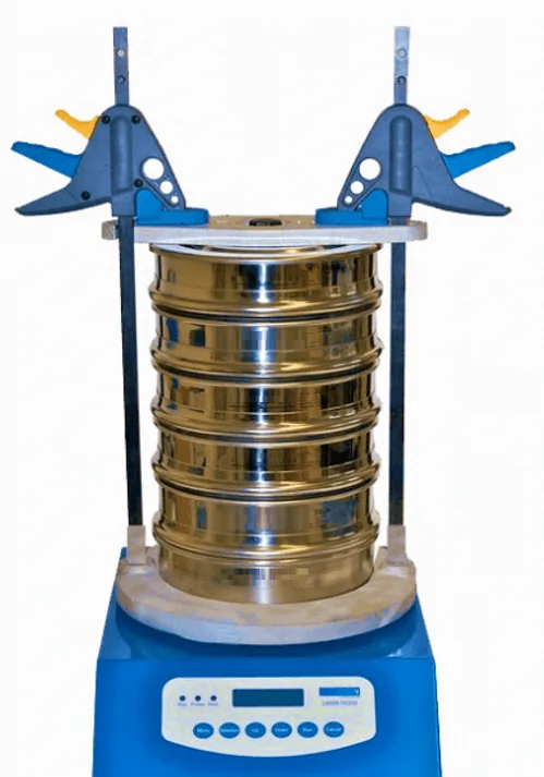
Screen analysis, also known as sieve analysis or particle size analysis, is a method used to determine the particle size distribution of a granular material. This process involves passing the material through a series of sieves with progressively smaller mesh sizes to separate and classify the particles based on their size.
There are two methods of screen analysis / sieve analysis to interpret the particle size distribution i.e Differential Analysis and Cumulative Analysis.
Differential Analysis also known as incremental analysis, the mass fraction of particles retained on each individual sieve is calculated. Distribution of particles are measured in histogram which shows the percentage of the total sample that is retained on each specific sieve size.
In Cumulative Analysis, the particle size distribution are measured in terms of the cumulative percentage of material that passes through or is retained by a specific sieve size. It tells how much of the total sample has a particle size smaller than or larger than each sieve size.
Related: Sphericity Calculator for different shapes
Screen Analysis Calculator for Differential and Cumulative Distribution
This Screen Analysis Tool helps to plot the particle size distribution based on Differential and Cumulative Analysis. In the table given below column of mesh data, including mesh size, screen opening, and mass fraction retained are given which user can change and see the output from the calculated data.
Note: The chart updates in real-time based on the input data, which then provides the visual representation of the average particle size distribution and cumulative analysis.
How to Use this Calculator : User can update the values present in the first 3 columns – Mesh, Screen Opening and Mass Fraction retained. To make this calculator more versatile, we have used the standard screen sizes.
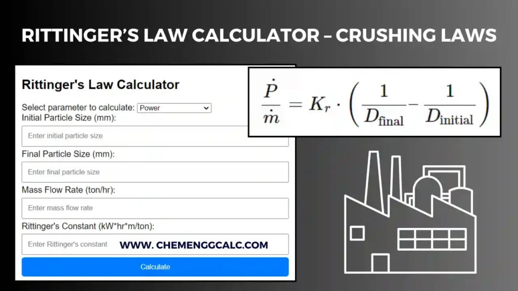
Related: Rittinger’s Law Calculator
Related: Kick’s Law Calculator
Related: Sphericity Calculator for different shapes
Python Code for Screen Analysis
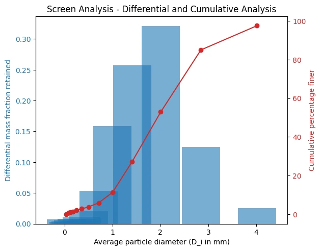
This python code helps user to perform a screen analysis on a dataset that represents particle size distribution. The plot helps visualize the distribution of particle sizes in terms of both differential and cumulative analysis.
import pandas as pd
import numpy as np
import matplotlib.pyplot as plt

# Define the data
data = {
    "Mesh": [4, 6, 8, 10, 14, 20, 28, 35, 48, 65, 100, 150, 200, 'Pan'],
    "Screen Opening (D_i in mm)": [4.6990, 3.3270, 2.3620, 1.6510, 1.1680, 0.8330, 0.5890, 0.4178, 0.2950, 0.2080, 0.1470, 0.1040, 0.0740, 0.0000],
    "Mass fraction retained (x_i)": [0.0000, 0.0251, 0.1250, 0.3207, 0.2570, 0.1590, 0.0538, 0.0210, 0.0102, 0.0077, 0.0058, 0.0041, 0.0031, 0.0075],
    "Average particle diameter (D_i in mm)": [np.nan, 4.0130, 2.8445, 2.0065, 1.4095, 1.0005, 0.7110, 0.5034, 0.3564, 0.2515, 0.1775, 0.1255, 0.0890, 0.0370]
}

# Create a DataFrame
df = pd.DataFrame(data)

# Calculate cumulative mass fraction retained
df['Cumulative mass fraction retained'] = df['Mass fraction retained (x_i)'].cumsum()

# Calculate cumulative percentage finer
df['Cumulative percentage finer'] = (1 - df['Cumulative mass fraction retained']) * 100

# Differential and Cumulative Analysis Plot
fig, ax1 = plt.subplots()

color = 'tab:blue'
ax1.set_xlabel('Average particle diameter (D_i in mm)')
ax1.set_ylabel('Differential mass fraction retained', color=color)
ax1.bar(df['Average particle diameter (D_i in mm)'], df['Mass fraction retained (x_i)'], color=color, alpha=0.6)
ax1.tick_params(axis='y', labelcolor=color)

ax2 = ax1.twinx()
color = 'tab:red'
ax2.set_ylabel('Cumulative percentage finer', color=color)
ax2.plot(df['Average particle diameter (D_i in mm)'], df['Cumulative percentage finer'], color=color, marker='o')
ax2.tick_params(axis='y', labelcolor=color)

fig.tight_layout()
plt.title('Screen Analysis - Differential and Cumulative Analysis')
plt.show()
Output:
Standard Screen Sizes (Mesh Number conversion)
Standard Screens are used to measure the size and the distribution of particles in the size range between about 3 and 0.0015 inches (76 \(\text{mm}\) and 38 \(\mu\text{m}\)).
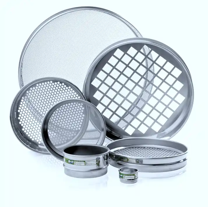
Testing sieves are made up of woven wire screens, the mesh and dimensions of standards mentioned below. The opening in each screen is square and identified as meshed per inch, however the actual opening of mesh is smaller due to certain thickness of wire.
As per Tyler standard screen series which is based on 200-mesh screen (equivalent to 0.074mm).
The area of openings in any of the screen is exactly the twice to that of opening in the next smaller screen.
Edition: 7th Edition, By: Warren L. McCabe, Julian C. Smith, Peter Harriott
A comprehensive resource on chemical engineering principles, covering core unit operations and practical applications essential for professionals and students alike.
Buy on AmazonHere is the table provide for standard screen with their mesh number and conversions in Inches, mm and Microns.
| US Sieve Size | Tyler Equivalent | Opening | ||
| mm | inch | Microns | ||
| – | 2½ Mesh | 8 | 0.312 | 8000 |
| – | 3 Mesh | 6.73 | 0.265 | 6730 |
| No. 3½ | 3½ Mesh | 5.66 | 0.233 | 5660 |
| No. 4 | 4 Mesh | 4.76 | 0.187 | 4760 |
| No. 5 | 5 Mesh | 4 | 0.157 | 4000 |
| No. 6 | 6 Mesh | 3.36 | 0.132 | 3360 |
| No. 7 | 7 Mesh | 2.83 | 0.111 | 2830 |
| No. 8 | 8 Mesh | 2.38 | 0.0937 | 2380 |
| No.10 | 9 Mesh | 2 | 0.0787 | 2000 |
| No. 12 | 10 Mesh | 1.68 | 0.0661 | 1680 |
| No. 14 | 12 Mesh | 1.41 | 0.0555 | 1410 |
| No. 16 | 14 Mesh | 1.19 | 0.0469 | 1190 |
| No. 18 | 16 Mesh | 1 | 0.0394 | 1000 |
| No. 20 | 20 Mesh | 0.841 | 0.0331 | 841 |
| No. 25 | 24 Mesh | 0.707 | 0.0278 | 707 |
| No. 30 | 28 Mesh | 0.595 | 0.0234 | 595 |
| No. 35 | 32 Mesh | 0.5 | 0.0197 | 500 |
| No. 40 | 35 Mesh | 0.42 | 0.0165 | 420 |
| No. 45 | 42 Mesh | 0.354 | 0.0139 | 354 |
| No. 50 | 48 Mesh | 0.297 | 0.0117 | 297 |
| No. 60 | 60 Mesh | 0.25 | 0.0098 | 250 |
| No. 70 | 65 Mesh | 0.21 | 0.0083 | 210 |
| No. 80 | 80 Mesh | 0.177 | 0.007 | 177 |
| No.100 | 100 Mesh | 0.149 | 0.0059 | 149 |
| No. 120 | 115 Mesh | 0.125 | 0.0049 | 125 |
| No. 140 | 150 Mesh | 0.105 | 0.0041 | 105 |
| No. 170 | 170 Mesh | 0.088 | 0.0035 | 88 |
| No. 200 | 200 Mesh | 0.074 | 0.0029 | 74 |
| No. 230 | 250 Mesh | 0.063 | 0.0025 | 63 |
| No. 270 | 270 Mesh | 0.053 | 0.0021 | 53 |
| No. 325 | 325 Mesh | 0.044 | 0.0017 | 44 |
| No. 400 | 400 Mesh | 0.037 | 0.0015 | 37 |
Related: Ergun Equation Calculator for Pressure Drop in Packed Bed Column
Related: Head Loss or Pressure Loss Calculator using Darcy-Weisbach Equation
Resources
- “Unit Operations in Chemical Engineering” (McCabe et al.)
- “Particle Technology and Separation Processes” (Richardson et al.)
- “Chemical Engineering Design: Principles, Practice and Economics of Plant and Process Design” (Towler and Sinnott)
Disclaimer: The Solver provided here is for educational purposes. While efforts ensure accuracy, results may not always reflect real-world scenarios. Verify results with other sources and consult professionals for critical applications. Contact us for any suggestions or corrections


