Table of Contents
The reaction rate constant also known as reaction rate coefficient (denoted as \(k\)), is a proportionality constant in chemical kinetics that relates the rate of a chemical reaction to the molar concentration of the reactants.
For a general chemical reaction represented as
aA + bB ⟶ cC + dD
the rate can be expressed as:
Rate = k [A]a. [B]b
Here, [A] and [B] are the molar concentrations of the reactants, and (a) and (b) are the orders of the reaction with respect to each reactant, which are determined experimentally.
Related: Performance Equation for Ideal Batch Reactor
Related: Rate Constant Calculation using Arrhenius Equation Calculator
Rate Constant Calculator for Zeroth, First and Second Order
This Rate Constant web calculator helps user to determine the rate constant of a chemical reaction based on time and concentration data. Then plots the data according to the Integrated Rate Equation which computes the rate constant and the value of R-Square which represents the best fit of the data.
To find out the order of the reaction, the value of R-Square should be close to 1 ensuring best fit of the data. Check the value of R-Square iteratively by selecting the order of the reaction.
Related: Arrhenius Activation Energy Calculator for two temperatures
Related: Performance Equation for Mixed Flow Reactor
How to use Rate Constant Calculator
- Input the Raw Data – Enter the values of time in “Time” column and concentration in corresponding “Concentration” column. By default, six rows are provided, by pressing “Add Row” more rows can be added in the input data field.
- Select Reaction Order – Choose the reaction order from the dropdown menu (Zeroth, First and Second Order), and simultaneously viewing the value of R-Square, which provides the best fit of the input data.
- For Zeroth Order- conc. vs time
- For First Order – ln (conc.) vs time
- For Second Order – 1/conc. vs time
- Viewing the Results and Plot Analyzing – The result section showing the calculated rate constant based on the slope calculated from the plot.
Integrated Rate Equation for Zeroth Order Reaction
For a zeroth-order reaction, the rate of reaction is given by:
\[ \text{Rate} = k \]
where \( k \) is the rate constant.
For a reactant \( A \) with concentration \([A]\), the rate can be expressed as:
\[ -\frac{d[A]}{dt} = k \]
Here negative sign indicates that the concentration of \( A \) decreases over time.
Now separating the variables to integrate with respect to time \( t \):
\[ \int \frac{d[A]}{dt} \, dt = \int -k \, dt \]
The integral of \(\frac{d[A]}{dt}\) with respect to \( t \) gives \([A]\):
\[ [A] = -kt + C \]
where \( C \) is the integration constant
To find the constant \( C \), use the initial condition. Let \([A]_0\) be the initial concentration of \( A \) at \( t = 0 \):
\[ [A]_0 = -k(0) + C \] \[ C = [A]_0 \]
Substitute \( C \) back into the integrated equation:
\[ [A] = -kt + [A]_0 \]
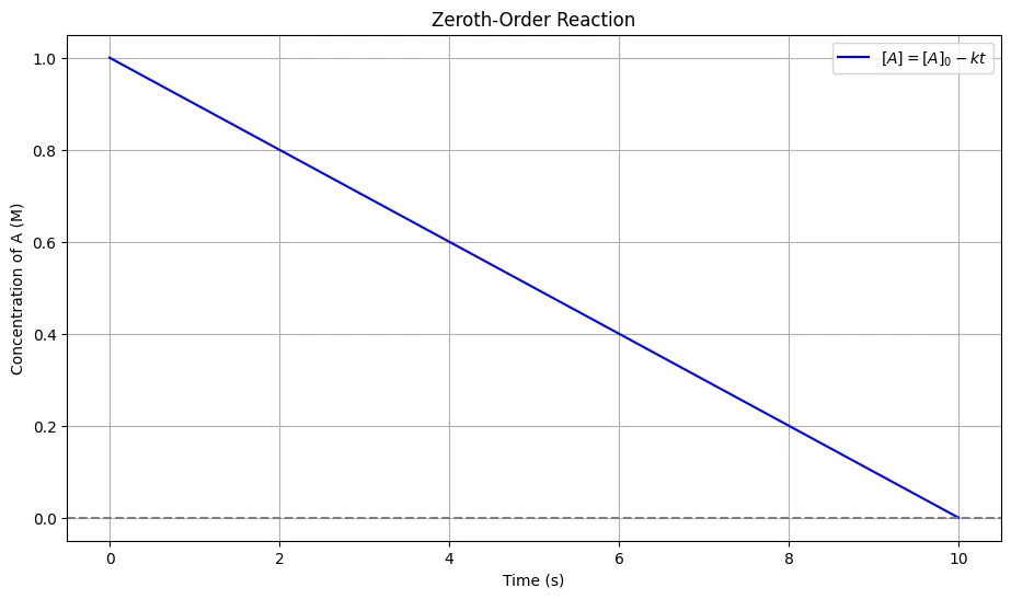
This is the zeroth-order integrated rate equation, which shows how the concentration of the reactant \( A \) changes with time \( t \). This equation indicates that the concentration of the reactant decreases linearly with time for a zeroth-order reaction.
Integrated Rate Equation for First Order Reaction
For a first-order reaction, the rate of reaction is given by:
\[ \text{Rate} = k[A] \]
where \( k \) is the rate constant and \([A]\) is the concentration of the reactant.
For a reactant \( A \) with concentration \([A]\), the rate can be expressed as:
\[ -\frac{d[A]}{dt} = k[A] \]
here negative sign indicates that the concentration of \( A \) decreases over time.
Separating variables to integrate with respect to time \( t \):
\[ \frac{d[A]}{[A]} = -k \, dt \]
now integrating both sides:
\[ \int \frac{1}{[A]} \, d[A] = \int -k \, dt \]
The integral of \(\frac{1}{[A]}\) with respect to \([A]\) is \(\ln[A]\), and the integral of \(-k\) with respect to \( t \) is \(-kt\):
\[ \ln[A] = -kt + C \]
where \( C \) is the integration constant.
To find the constant \( C \), use the initial condition. Let \([A]_0\) be the initial concentration of \( A \) at \( t = 0 \):
\[ \ln[A]_0 = -k(0) + C \] \[ C = \ln[A]_0 \]
Now, substituting \( C \) back into the integrated equation:
\[ \ln[A] = -kt + \ln[A]_0 \]
Above equation can be rearranged to:
\[ \ln\left(\frac{[A]}{[A]_0}\right) = -kt \]
or, taking exponent both side
\[ \frac{[A]}{[A]_0} = e^{-kt} \]
\[ [A] = [A]_0 e^{-kt} \]
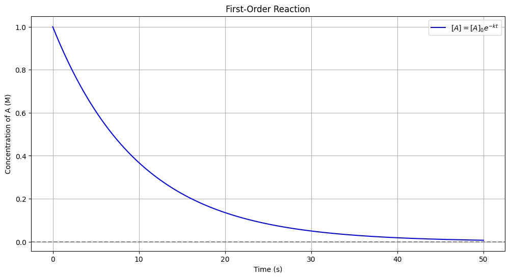
This equation indicates that the concentration of the reactant decreases exponentially with time for a first-order reaction.
Integrated Rate Equation for Second Order Reaction
For a second-order reaction, the rate of reaction is given by:
\[ \text{Rate} = k[A]^2 \] where \( k \) is the rate constant and \([A]\) is the concentration of the reactant.
For a reactant \( A \) with concentration \([A]\), the rate can be expressed as:
\[ -\frac{d[A]}{dt} = k[A]^2 \]
Here negative sign indicates that the concentration of \( A \) decreases over time.
Separate the variables to integrate with respect to time \( t \):
\[ \frac{d[A]}{[A]^2} = -k \, dt \]
Integrating both sides:
\[ \int \frac{1}{[A]^2} \, d[A] = \int -k \, dt \]
The integral of \(\frac{1}{[A]^2}\) with respect to \([A]\) is \(-\frac{1}{[A]}\), and the integral of \(-k\) with respect to \( t \) is \(-kt\):
\[ -\frac{1}{[A]} = -kt + C \]
where \( C \) is the integration constant.
To find the constant \( C \), use the initial condition. Let \([A]_0\) be the initial concentration of \( A \) at \( t = 0 \):
\[ -\frac{1}{[A]_0} = -k(0) + C \] \[ C = -\frac{1}{[A]_0} \]
Substituting \( C \) back into the integrated equation:
\[ -\frac{1}{[A]} = -kt – \frac{1}{[A]_0} \]
above equation can be rewritten as
\[ \frac{1}{[A]} = kt + \frac{1}{[A]_0} \]
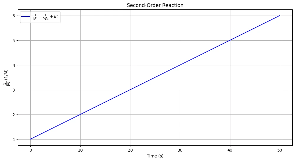
This equation indicates that the inverse of the concentration of the reactant increases linearly with time for a second-order reaction.
Python Code for Reaction Rate Constant
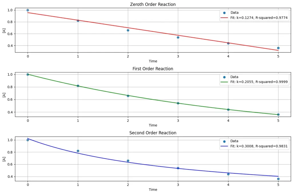
This Python code analyzes reaction kinetics by fitting experimental data to models representing zeroth, first, and second-order reactions. The result plots how the concentration of a reactant changes over time for each reaction order.
Note: This Python code solves the specified problem for 1st order reaction. Users can copy the code and run it in a suitable Python environment. By adjusting the input parameters, and observe how the output changes accordingly.
import numpy as np
import matplotlib.pyplot as plt
from scipy.optimize import curve_fit

# Sample data: Time (t) and concentration ([A])
time = np.array([0, 1, 2, 3, 4, 5])  # Example time data
concentration = np.array([1.0, 0.82, 0.66, 0.54, 0.44, 0.36])  # Example concentration data

# Define functions for each reaction order
def zeroth_order(t, k, A0):
    return A0 - k * t

def first_order(t, k, A0):
    return A0 * np.exp(-k * t)

def second_order(t, k, A0):
    return 1 / (1 / A0 + k * t)

# Initial guess for the parameters [k, A0]
initial_guess = [0.1, concentration[0]]

# Fit the data to each model
popt_zeroth, _ = curve_fit(zeroth_order, time, concentration, p0=initial_guess)
popt_first, _ = curve_fit(first_order, time, concentration, p0=initial_guess)
popt_second, _ = curve_fit(second_order, time, concentration, p0=initial_guess)

# Generate points for plotting the fitted curves
time_fit = np.linspace(min(time), max(time), 100)
conc_fit_zeroth = zeroth_order(time_fit, *popt_zeroth)
conc_fit_first = first_order(time_fit, *popt_first)
conc_fit_second = second_order(time_fit, *popt_second)

# Calculate R-squared values
def r_squared(y_data, y_fit):
    residual = y_data - y_fit
    ss_residual = np.sum(residual ** 2)
    ss_total = np.sum((y_data - np.mean(y_data)) ** 2)
    r2 = 1 - (ss_residual / ss_total)
    return r2

r_squared_zeroth = r_squared(concentration, zeroth_order(time, *popt_zeroth))
r_squared_first = r_squared(concentration, first_order(time, *popt_first))
r_squared_second = r_squared(concentration, second_order(time, *popt_second))

# Plotting the data and the fitted curves
plt.figure(figsize=(12, 8))

# Plot for Zeroth Order Reaction
plt.subplot(3, 1, 1)
plt.scatter(time, concentration, label='Data')
plt.plot(time_fit, conc_fit_zeroth, label=f'Fit: k={popt_zeroth[0]:.4f}, R-squared={r_squared_zeroth:.4f}', color='red')
plt.title('Zeroth Order Reaction')
plt.xlabel('Time')
plt.ylabel('[A]')
plt.legend()
plt.grid(True)

# Plot for First Order Reaction
plt.subplot(3, 1, 2)
plt.scatter(time, concentration, label='Data')
plt.plot(time_fit, conc_fit_first, label=f'Fit: k={popt_first[0]:.4f}, R-squared={r_squared_first:.4f}', color='green')
plt.title('First Order Reaction')
plt.xlabel('Time')
plt.ylabel('[A]')
plt.legend()
plt.grid(True)

# Plot for Second Order Reaction
plt.subplot(3, 1, 3)
plt.scatter(time, concentration, label='Data')
plt.plot(time_fit, conc_fit_second, label=f'Fit: k={popt_second[0]:.4f}, R-squared={r_squared_second:.4f}', color='blue')
plt.title('Second Order Reaction')
plt.xlabel('Time')
plt.ylabel('[A]')
plt.legend()
plt.grid(True)

plt.tight_layout()
plt.show()
Output:
Resources
- Chemical Reactor Analysis and Design Fundamentals by Rawlings and Ekerdt
- Elements of Chemical Reaction Engineering by Fogler
- “Chemical Reaction Engineering“ by Octave Levenspiel
Disclaimer: The Solver provided here is for educational purposes. While efforts ensure accuracy, results may not always reflect real-world scenarios. Verify results with other sources and consult professionals for critical applications. Contact us for any suggestions or corrections.

