Table of Contents
Distillation is the most commonly used unit operation in chemical engineering, widely applied for the separation and purification of liquid mixtures. The Ponchon-Savarit method provides a detailed graphical approach for designing binary distillation columns by incorporating both mass and energy balances.
The main purpose of the Ponchon-Savarit method is to determine the theoretical number of stages required for separation by simultaneously considering both material and enthalpy balances, making it more accurate for systems with significant energy effects.
Related: 15 Mostly used Fundamental Constants Every Chemical Engineer Should Know
Ponchon-Savarit Diagram Calculator
This ChemEnggCalc Ponchon-Savarit Diagram Calculator is a web-based tool for designing binary distillation columns. It helps users visualize and analyze the separation of a binary mixture using the Ponchon-Savarit method.
Based on input parameters such as distillate composition (xD), bottoms composition (xB), feed composition (xF), feed quality (q), and enthalpy-composition data, the tool graphically calculates the number of theoretical stages, feed stage location, condenser and reboiler heat duties, and minimum reflux ratio.
Note: Insert your own enthalpy-composition data using the JSON format provided below. Make sure to include real data within the structure.
Related: Joule-Thomson Effect – Coefficient Calculation for CO2 and N2
Related: Interactive McCabe-Thiele Diagram Generator for Binary Distillation
Assumptions for Ponchon-Savarit Method
The Ponchon-Savarit method is a graphical technique for the design and analysis of binary distillation columns, it incorporates both material and energy balances. This method is based on a set of assumptions to simplify the calculations and diagram construction. Here are the following assumptions:
- Binary Mixture: The method is applicable only to binary systems (two-component mixtures).
- Enthalpy-Composition Data: Accurate enthalpy vs. composition data is used for both liquid and vapor phases, allowing for energy balance analysis.
- Equilibrium Stages: Each theoretical stage is assumed to achieve complete vapor-liquid equilibrium.
- Adiabatic Column: The distillation column is considered adiabatic, meaning there is no heat loss to the surroundings, except at the condenser and reboiler.
- No Side Streams or Reactions: There are no side streams, azeotropes, or chemical reactions involved in the system.
- Variable Molar Overflow Allowed: Unlike McCabe-Thiele, the Ponchon-Savarit method does not assume constant molar overflow, making it suitable for systems with significant energy effects or non-linear enthalpy behavior.

Related: Importance of Programming and Coding in Chemical Engineering
Related: 10 Mostly used Dimensionless Numbers in Chemical Engineering
How to Use Ponchon-Savarit Diagram Calculator
This Ponchon-Savarit Calculator tool is easy to use. Follow the steps below to generate the plot and results table. By default, sample data is preloaded, which can be modified as needed.
Step 1. Input Process Parameters:
Enter the feed composition (z_F, 0–1), flow rate (F, kmol/hr), distillate composition (x_D, 0–1), bottoms composition (x_W, 0–1), feed thermal condition (q, 0–1), and reflux ratio (R, ≥0) in the input fields.
Step 2. Provide VLE and Enthalpy Data:
In the textarea labeled “VLE and Enthalpy Data (JSON format),” input a JSON object containing enthalpy-composition diagram data. You may use the default data or replace it.
Important! Ensure the data is structured exactly as shown below to avoid parsing errors:
{
"xData": [0, 0.08, 0.18, 0.25, 0.49, 0.65, 0.79, 0.91, 1.0],
"yData": [0, 0.28, 0.43, 0.51, 0.73, 0.83, 0.90, 0.96, 1.0],
"Hl": [24.3, 24.1, 23.2, 22.8, 22.05, 21.75, 21.7, 21.6, 21.4],
"Hv": [61.2, 59.6, 58.5, 58.1, 56.5, 55.2, 54.4, 53.8, 53.3]
}
Ensure that the arrays of liquid and vapour mole fractions range from 0 to 1 and are monotonically increasing.
Step 3. Load JSON Data:
Click the “Load JSON Data” button to validate and apply the VLE and enthalpy data. A status message will confirm successful loading or indicate errors if the JSON is invalid.
Step 4. Review Results
View the interactive enthalpy-composition plot and results table showing the number of stages, feed stage location, heat duties, and minimum reflux ratio.
Note: Users may also access this calculator from this link – https://chemenggcalc.github.io/Ponchon-savarit-calculator/
Also Read: Convective Mass Transfer Coefficient – Concept and Calculation
Also Read: Fick’s First Law of Diffusion Calculator – Molecular Diffusion
Ponchon-Savarit Diagram Generator – Python Code
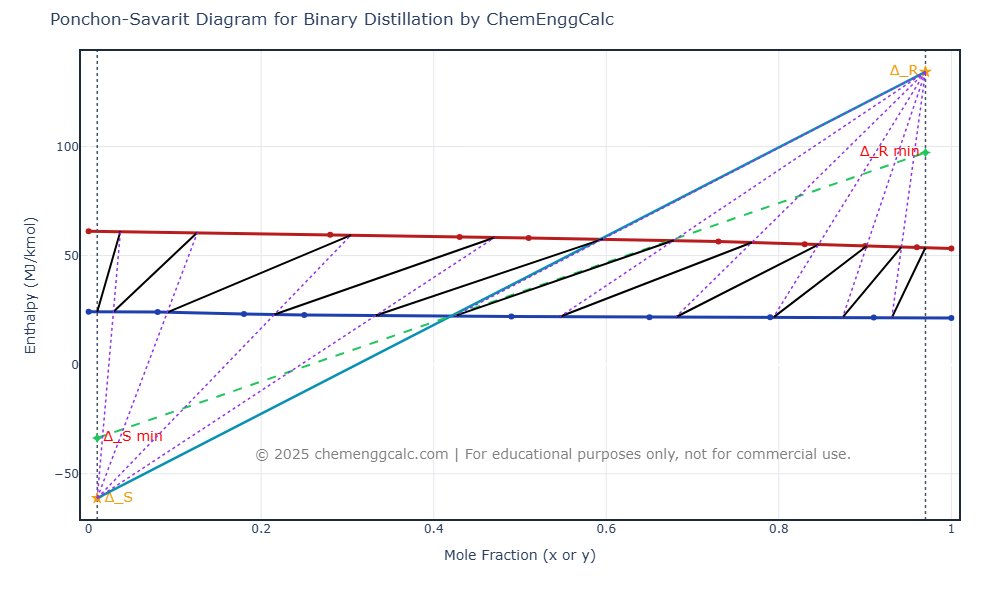
This Python code for the Ponchon-Savarit diagram calculator is used to plot the enthalpy-composition diagram and calculate operating conditions such as the number of theoretical stages, feed stage location, and heat duties in a binary distillation column using the Ponchon-Savarit method.
Note: This code is written for the Google Colab environment. You can directly access the code by clicking the link provided – Ponchon-Savarit Diagram Generator.
Users can edit the code by copying the script and modifying the input parameters such as compositions, feed quality, and enthalpy data to observe their effects on the separation process and output results.
Output:
| Parameter | Value | Unit |
|---|---|---|
| Distillate Flow Rate (D) | 4.27 | kmol/hr |
| Bottoms Flow Rate (W) | 5.73 | kmol/hr |
| Rectifying Difference Point (Δ_R) | (0.97, 134.20) | (Mole fraction, MJ/kmol) |
| Stripping Difference Point (Δ_S) | (0.01, -61.17) | (Mole fraction, MJ/kmol) |
| Condenser Duty (Q_C) | 133.74 | kW |
| Reboiler Duty (Q_R) | 135.98 | kW |
| Δ_R min (x_D, Q’_min) | (0.97, 97.39) | (Mole fraction, MJ/kmol) |
| Δ_S min (x_W, Q”_min) | (0.01, -33.73) | (Mole fraction, MJ/kmol) |
| Minimum Reflux Ratio (R_min) | 1.36 | Dimensionless |
| Number of Theoretical Stages | 11 (Feed Stage: 7) | Dimensionless |
| Stage 1 | x: 0.932, y: 0.970 | Mole fraction |
| Stage 2 | x: 0.876, y: 0.943 | Mole fraction |
| Stage 3 | x: 0.796, y: 0.903 | Mole fraction |
| Stage 4 | x: 0.683, y: 0.847 | Mole fraction |
| Stage 5 | x: 0.550, y: 0.771 | Mole fraction |
| Stage 6 | x: 0.428, y: 0.681 | Mole fraction |
| Stage 7 | x: 0.336, y: 0.599 | Mole fraction |
| Stage 8 | x: 0.218, y: 0.476 | Mole fraction |
| Stage 9 | x: 0.093, y: 0.308 | Mole fraction |
| Stage 10 | x: 0.030, y: 0.129 | Mole fraction |
| Stage 11 | x: 0.010, y: 0.038 | Mole fraction |
Resources
- “Transport Phenomena” by R. Byron Bird, Warren E. Stewart, and Edwin N. Lightfoot.
- “Introduction to Chemical Engineering Thermodynamics” by J.M. Smith, H.C. Van Ness, and M.M. Abbott.
- “Mass Transfer Operations” by Robert E. Treybal.
Disclaimer: The Solver provided here is for educational purposes. While efforts ensure accuracy, results may not always reflect real-world scenarios. Verify results with other sources and consult professionals for critical applications. Contact us for any suggestions or corrections.