Table of Contents
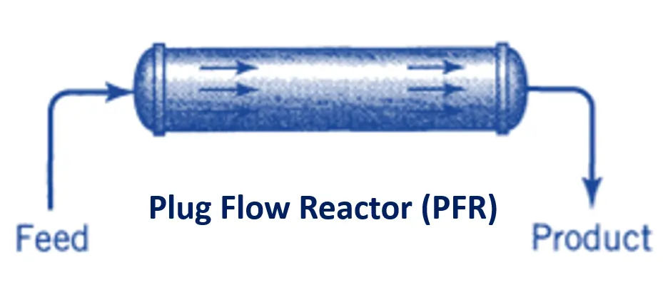
A plug flow reactor (PFR), also sometimes called a continuous tubular reactor (CTR) or piston flow reactor, is a model used to describe chemical reactions in continuous, flowing systems with a cylindrical geometry. In a plug flow reactor the composition of the fluid varies from point to point along a flow path and having negligible radial mixing.
In a PFR, the reactants enter at one end of the reactor and flow through it continuously, undergoing chemical reaction as they progress along the length of the reactor. PFRs are often used when precise control over residence time and reaction conditions is required, as they offer uniform reaction conditions and allow for the study of kinetics and reaction mechanisms.
Space-Time and Space-Velocity
Space-time (\(\tau\)) and space-velocity (s) are key performance metrics for flow reactors.
Space-Time (\(\tau\)) is defined as the time required to process one reactor volume of feed measured at specified conditions. It is measured in time (hours or minutes or seconds). A space-time of 5 min means that every 5 min one reactor volume of feed at specified conditions is being treated by the reactor.
\(\tau = \frac{1}{s}\) where, s is the space time.
Space-Velocity (s) is the number of reactor volumes of feed at specified conditions which can be treated at one unit time. It is measured in time-1 (hour-1or minute-1or sec-1). A space-velocity of 2 hr-l means that two reactor volumes of feed at specified conditions are being fed into the reactor per hour.
\(s = \frac{1}{\tau}\) where, \(\tau\) is the space-time.
The values of space-time and space-velocity depends on the conditions selected. If they are of the stream entering the reactor, the relation between s and r and the other pertinent variables is
\[\tau = \frac{1}{s} = \frac{C_{A0}V}{F_{A0}} = \frac{V}{{v_0}}\]
where, \(C_{A0}\) is initial concentration of component A (mol/liter), V is the reactor volume (liter), \(F_{A0}\) Initial molar flow rate of component A (mol/time), \(v_0\) is the volumetric feed rate (liter/time).
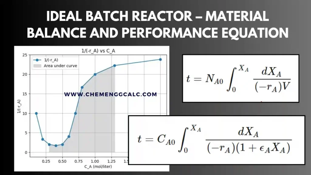
Related: Performance Equation for Ideal Batch Reactor
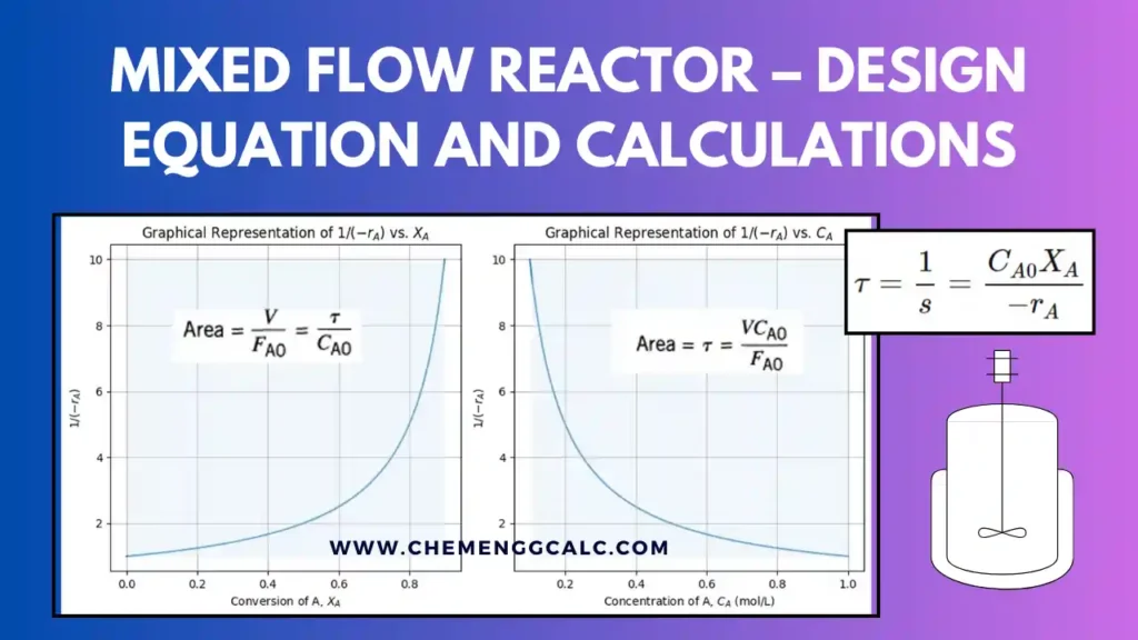
Related: Performance Equation for Mixed Flow Reactor
Design Equation for Plug Flow Reactor
The starting point for all design is the material balance expressed for any reactant (or product). In case of plug flow reactor the composition of the fluid varies from point to point along a flow path.
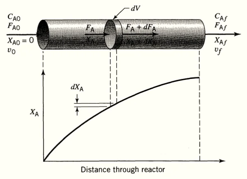
The material balance for a reaction component must be made for a differential element of volume dV. Thus for reactant A,
Input = Output + Disappearance +Accumulation------- Eq 1
Accumulation = 0 , for steady state
Input of \( A \) (moles/time) = \( F_{A} \)
Output of \( A \) (moles/time) = \( F_A + dF_A\)
Disappearance of \( A \) by reaction (moles/time) = \( (-r_A)dV \) , where \(-r_A\) is rate of reaction with respect to component A
putting these terms in equation 1, we get:
\[F_A = (F_A + dF_A) + (-r_A) dV\]
by putting the value of \( F_A = F_{A0} (1-X_A) \) , we get
\[F_{A0}dX_A = (-r_A) dV\]
Above equation accounts for reactant A in the differential section of reactor of volume dV. For the reactor as a whole the expression must be integrated:
\[\int_{0}^{V}\frac{dV}{F_{A0}} = \int_{0}^{X_{Af}}\frac{dX_A}{-r_A}\]
On Integration, we get:
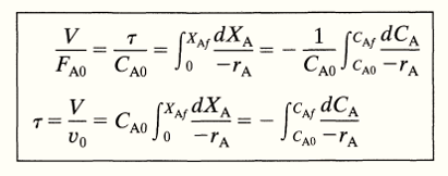
\[\frac{V}{F_{A0}} = \frac {\tau}{C_{A0}} = \int_{0}^{X_{Af}}\frac{dX_A}{-r_A}\] —- Eq 2
where, \(\tau\) is the space time
Rearranging the Eq 2 for any value of \(\varepsilon\)
\[ \tau = \frac{V}{v_0} = {C_{A0}} \int_{0}^{X_{Af}}\frac{dX_A}{-r_A}\] —- Eq 3
where:
- \(v_0\) = volumetric feed rate (liter/time)
- FA0 = Initial Flowrate (mol/time)
- XA = Extent of the reaction component (conversion) from 0 to 1
Eq 3 can be used to determine of reactor size for a given feed rate and required conversion. As a more general expression for plug flow reactors, if the feed on which conversion \((X_{Ai})\) is based, enters the reactor partially converted, and leaves at a desired conversion \((X_{Af})\), so we get,
\[\frac{V}{F_{A0}} = \int_{X_{Ai}}^{X_{Af}}\frac{dX_A}{-r_A}\]
For the constant density system i.e \(\varepsilon = 0\), where \(X_A = 1 – \frac{C_A}{C_{A0}}\) and on differentiating it, \(dX_A = -\frac{dC_A}{C_{A0}}\), the performance equation can be written in terms of concentration, putting \(dX_A\) in equation 3 we get:
\[\frac{V}{F_{A0}} = -\frac{1}{C_{A0}} \int_{C_{A0}}^{C_{Af}}\frac{dC_A}{-r_A}\]
or
\[\tau = \frac{V}{v_0} = -\int_{C_{A0}}^{C_{Af}}\frac{dC_A}{-r_A}\]
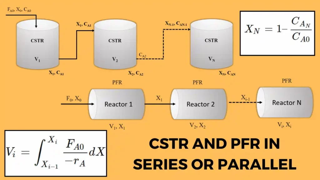
Related: PFR and CSTR in Series or Parallel Combination for a single reaction
Must Read: Personal Carbon Footprint Calculator – Track your CO2 Emissions
Python Code for Plug Flow Reactor
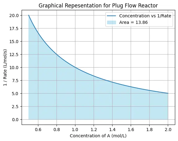
This python code computes the behavior of a chemical reaction within a plug flow reactor. User first put the values of initial concentration \(C_{A0}\) and final concentration \(C_{Af}\) of the reactant A at the given conditions of initial molar flow rate and reactor volume. The rate of the reaction can be changed by the user, we have solved it for first order taking as \(-k.C_A\)
Based on the given data the code produce data points are then plotted, with A concentration on the x-axis and the reciprocal of the reaction rate \(\frac{1}{rate}\) on the y-axis. The area under the curve using the trapezoidal rule and highlights the value of \(𝐶_{𝐴0}\frac{𝑉}{𝐹_{𝐴0}}\) on the plot.
Note: This Python code solves the specified problem for 1st order reaction. Users can copy the code and run it in a suitable Python environment. By adjusting the input parameters, and observe how the output changes accordingly.
import numpy as np
import matplotlib.pyplot as plt
from scipy.integrate import trapz

# Define constants
CA0 = 2.0  # Initial concentration of A (mol/L)
CAf = 0.5  # Final concentration of A (mol/L)
V_over_FA0 = 5.0  # Just an example value for CA0 * V / FA0

# Define the rate expression function
def rate_expression(CA):
    # Example rate expression: -k * CA
    k = 0.1  # Rate constant (1/s)
    return k * CA**1

# Generate concentration values
CA_values = np.linspace(CAf, CA0, 100)

# Calculate corresponding rates
rates = [rate_expression(CA) for CA in CA_values]

# Calculate 1/rate
one_over_rates = [1 / rate if rate != 0 else np.inf for rate in rates]

# Plot concentration vs 1/rate
plt.plot(CA_values, one_over_rates, label='Concentration vs 1/Rate')
plt.xlabel('Concentration of A (mol/L)')
plt.ylabel('1 / Rate (L/mol/s)')

# Area under the curve
area = trapz(one_over_rates, CA_values)
plt.fill_between(CA_values, one_over_rates, color='skyblue', alpha=0.5, label=f'Area = {area:.2f}')

plt.title('Plug Flow Reactor: Concentration vs 1/Rate')
plt.grid(True)
plt.legend()
plt.show()
Output:
Example Problem on Plug Flow Reactor
A specific enzyme acts as catalyst in the fermentation of reactant A. At a given enzyme concentration in the aqueous feed stream (25 \(\frac{liter}{min}\)) find the volume of plug flow reactor needed for 95% conversion of reactant A (2 \(\frac{mol}{liter}\)). The kinetics of the fermentation at this enzyme concentration is given by
A ——> R (Enzymatic Reaction)
\(-r_A = \frac{0.1C_A}{1 + 0.5C_A} \frac{mol}{liter.min}\) ?
Given:
- conversion for reactant A, \(X_A\) = 0.95
- Volumetric Feed Rate, \(v_0\) = 25 liter/min
- Initial concentration of feed, \(C_{A0}\) = 2 mol/liter
- Volume of Reactor, \(V\) = ?
based on the given information, first we will find CA
\(C_{Af} = C_{A0}(1−X_A)\)
C_{Af} = 2 * (1 – 0.95) = 0.1 mol/liter
using performance equation for plug flow reactor,
\(\tau = \frac{V}{v_0} = -\int_{C_{A0}}^{C_{Af}}\frac{dC_A}{-r_A}\)
replacing the value of \(-r_A\) with the given rate of reaction and putting in above equation, we get
\(\tau = -\int_{C_{A0}}^{C_{Af}}\frac{0.1C_A}{1 + 0.5C_A} dC_A\)
on solving this equation we get,
\(\tau = 10 \ln \frac{C_{A0}}{C_A} + 5 (C_{A0} – C_A)\)
now, putting the values of \(C_{A0}\) and \(C_A\), we get the value of \(\tau\) as
\(\tau\) = 10 \( \ln \frac{2}{0.1} + 5 (2 – 0.1)\)
\(\tau\) = \(\frac{V}{v_0}\) = 39.4573 min
Therefore, \(V = 39.4573 * 25\)
\(V\) = 986.433 liters ~ 1m3
Resources:
- Chemical Reactor Analysis and Design Fundamentals by Rawlings and Ekerdt
- Elements of Chemical Reaction Engineering by Fogler
- “Chemical Reaction Engineering“ by Octave Levenspiel
Disclaimer: The Solver provided here is for educational purposes. While efforts ensure accuracy, results may not always reflect real-world scenarios. Verify results with other sources and consult professionals for critical applications. Contact us for any suggestions or corrections.


