Table of Contents
An Ideal batch reactor is a type of chemical reactor where reactants are mixed together in a closed vessel, and the reaction proceeds without any inflow or outflow of reactants during the reaction time.
In a batch reactor, the composition is uniform throughout at any instant of time, noting that no fluid enters or leaves the reaction mixture during reaction.
Material Balance for an Ideal Batch Reactor
The starting point for all design is the material balance expressed for any reactant (or product).
General Material Balance for any Reactor:
(Rate of Reactant flow into element of volume) = (Rate of Reactant flow out of element of volume) + (Rate of reactant loss due to chemical reaction within the element of the volume) + (Rate of accumulation of reactant in element of volume)
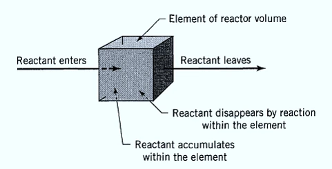
of the reactor
For the ideal batch reactor, the reactants are initially charged into a container, are well mixed, and are left to react for a certain period. The resultant mixture is then discharged. This is an unsteady-state operation where composition changes with time; however, at any instant the composition throughout the reactor is uniform.
input=output+ disappearance + accumulation
Let us make a material balance for any component A (assuming this component as limiting component) since the composition is uniform throughout at any instant of time, we may make the accounting about the whole reactor.
Thus we left with:
+(Rate of loss of reactant A within reactor due to chemical reaction) = - (Rate of accumulation of reactant A within the reactor)
The disappearance of \( A \) moles due to reaction can be expressed as \( (-r_A)V \), where \( V \) represents the volume of fluid.
The accumulation of \( A \) is given by the change in the number of moles with respect to time, represented by \( -\frac{{dN_A}}{{dt}} \). It gives the change in the initial number of moles \( [N_{Ao}(1 – X_A)] \) due to reaction progress \( X_A \).
Thus, the equation becomes:
\( \text{Disappearance rate of A} :\)
\(\frac{\text{moles of A reacting}}{\text{time} \times \text{volume}} \times \text{volume} \)
\( \text{Accumulation of } A:\)
\( -\frac{{dN_A}}{{dt}} = -\frac{{d[N_{Ao}(1 – X_A)]}}{{dt}}\)
\( = -N_{Ao} \frac{{dX_A}}{{dt}} \)
By putting these two terms we get,
\( (-r_A)V = N_{A0} \frac{dX_A}{dt} \) —— Eq 1
Rearranging and integrating then gives
\[ t = N_{A0} \int_{0}^{X_A} \frac{dX_A}{(-r_A)V} \] —— Eq 2
where:
- -rA = Rate of a Reaction for component A
- V = volume of the reactor (reaction volume)
- NA0 = Initial Moles of a reaction
- XA = Extent of the reaction component (conversion) from 0 to 1
Related: PFR and CSTR in Series or Parallel Combination for a single reaction
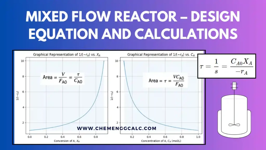
Related: Performance equation for Mixed Flow Reactor
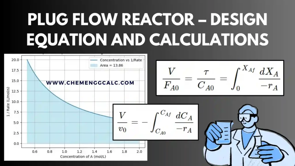
Related: Performance Equation for Plug Flow Reactor
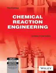
Edition: 3rd Edition, By: Octave Levenspiel
A classic textbook covering the principles of chemical reaction engineering with detailed analysis of reactor design and kinetics.
Buy on AmazonPerformance Equation / Design Equation of a Batch Reactor
Above equation is the general form (Eq 2) showing the time required to achieve a conversion \(X_A\) for either isothermal or non-isothermal operation. Further simplifying this for constant density of the fluid (constant volume system) i.e for \(( \varepsilon _A = 0\)), we get:
\[ t = C_{A0} \int_{0}^{X_A} \frac{dX_A}{-r_A} \]
In terms of concentration
\[ t = -\int_{C_{A0}}^{C_A} \frac{dC_A}{-r_A} \]
where CA0 is Concentration of component A
Now, for all those reactions in which the volume of reacting mixture changes proportionately with conversion, such as in single gas-phase reactions with significant density changes for \(( \varepsilon _A \neq 0 )\), we get:
\[ t = N_{A0} \int_{0}^{X_A} \frac{dX_A}{(-r_A) V_0 (1 + \epsilon_A X_A)} \]
which can be written as:
\[ t = C_{A0} \int_{0}^{X_A} \frac{dX_A}{(-r_A)(1 + \epsilon_A X_A)} \]
where, \(\varepsilon = \frac{{N_{A0} – N_A}}{{N_{A0}}}\)
Python Code for Batch Reactor for constant density \((\varepsilon_A = 0)\)
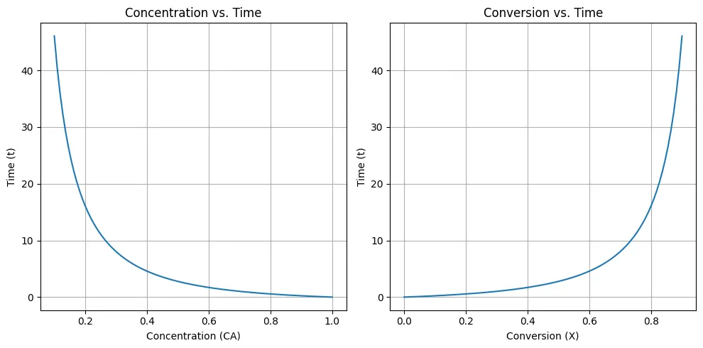
The code computes and provide plots for an ideal batch reactor when \((\varepsilon_A = 0)\). In the first plot the change in reactant concentration (CA) over time (t), and in second the relationship between conversion (X) and time (t). These plots gives insights into the kinetics of the reaction and the progress of the conversion process, optimizing reaction conditions for desired product yields.
Note: This Python code solves the specified problem for 1st order reaction. Users can copy the code and run it in a suitable Python environment. By adjusting the input parameters, and observe how the output changes accordingly.
import numpy as np
import matplotlib.pyplot as plt

# Define the concentration range
CA_range = np.linspace(0.1, 1, 100)

# Define the rate law (example)
def rate_law(CA):
    k = 0.5  # Rate constant
    return k * CA

# Calculate the reaction time and conversion for each concentration
t_values = []
X_values = []
for CA in CA_range:
    rA = rate_law(CA)
    t = -np.log(CA) / rA
    X = 1 - CA / CA_range[-1]  # Conversion definition
    t_values.append(t)
    X_values.append(X)

# Plotting concentration vs. time
plt.figure(figsize=(10, 5))
plt.subplot(1, 2, 1)
plt.plot(CA_range, t_values)
plt.title('Concentration vs. Time')
plt.xlabel('Concentration (CA)')
plt.ylabel('Time (t)')
plt.grid(True)

# Plotting conversion vs. time
plt.subplot(1, 2, 2)
plt.plot(X_values, t_values)
plt.title('Conversion vs. Time')
plt.xlabel('Conversion (X)')
plt.ylabel('Time (t)')
plt.grid(True)

plt.tight_layout()
plt.show()
Output:
Python Code for Batch Reactor for varying volume \(( \varepsilon _A \neq 0 )\)
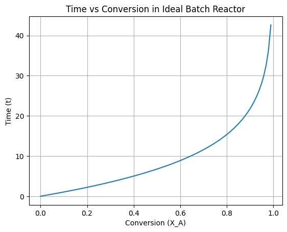
The code computes and provide plots for an ideal batch reactor when \((\varepsilon_A \neq 0)\). In this plot the change in reactant concentration (CA) over time (t).
Note: This Python code solves the specified problem for 1st order reaction. Users can copy the code and run it in a suitable Python environment. By adjusting the input parameters, and observe how the output changes accordingly.
import numpy as np
import matplotlib.pyplot as plt
from scipy.integrate import quad

# Function to define the rate of reaction (-r_A)
def rate_of_reaction(X_A):
    return k * C_A0*(1 - X_A)

# Function to define the integrand for the integral
def integrand(X_A):
    rate = rate_of_reaction(X_A)
    if rate == 0:
        return np.inf  # Return infinity to avoid division by zero
    else:
        return 1 / (rate * V_0 * (1 + epsilon_A * X_A))

# Constants
N_A0 = 1.0  # Initial moles of A
V_0 = 1.0   # Initial volume of the reactor (L)
k = 0.1     # Rate constant (L/mol/s)
epsilon_A = 0.1  # Molar flow rate constant
C_A0 = N_A0/V_0  # Initial Concentration

# Array of conversion values (0 to 1)
X_A_values = np.linspace(0, 1, 100)

# Calculate time for each conversion value
time_values = []
for X_A in X_A_values:
    # Perform the integral using quad function from scipy
    integral_value, _ = quad(integrand, 0, X_A)
    time_values.append(N_A0 * integral_value)

# Plotting
plt.plot(X_A_values, time_values)
plt.xlabel('Conversion (X_A)')
plt.ylabel('Time (t)')
plt.title('Time vs Conversion in Ideal Batch Reactor')
plt.grid(True)
plt.show()
Output:
Example Problem on Ideal Batch Reactor
We are planning to operate a batch reactor to convert A into R. This is a liquid reaction, the stoichiometry is 𝐴→𝑅, and the rate of reaction is given in Table. How long must we react each batch for the concentration to drop from 𝐶A0 = 1.3 mol/liter to 𝐶A𝑓 = 0.3 mol/liter?
| CA (mol/liter) | -rA (mol/liter⋅min) |
|---|---|
| 0.1 | 0.1 |
| 0.2 | 0.3 |
| 0.3 | 0.5 |
| 0.4 | 0.6 |
| 0.5 | 0.5 |
| 0.6 | 0.25 |
| 0.7 | 0.10 |
| 0.8 | 0.06 |
| 1 | 0.05 |
| 1.3 | 0.045 |
| 2 | 0.042 |
Given:
- CA0 = 1.3 mol/liter
- CAf = 0.3 mol/liter
Reaction : A ———-> R
No change in the stoichiometry \((\varepsilon_A = 0)\)
Using the performance equation of the batch reactor for \((\varepsilon_A = 0)\)
\( t = -\int_{C_{A0}}^{C_A} \frac{dC_A}{-r_A} \)
Now, making the plots for 1/(-rA) vs CA

putting the values in the performance equation, we get:
\( t = -\int_{0.3}^{1.3} \frac{dC_A}{-r_A} \)
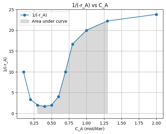
Above plot showing the graphical representation for ideal batch reactor. Therefore, the area under the curve give the integration value.
Hence, time = Area under the curve which is 12.7
Python code to solve this integration, you can also solve it by hand using Numerical integration using the trapezoidal rule.
import numpy as np
from scipy.integrate import trapz

# Provided data
C_A = np.array([0.1, 0.2, 0.3, 0.4, 0.5, 0.6, 0.7, 0.8, 1, 1.3, 2])  # Concentration (mol/liter)
minus_r_A = np.array([0.1, 0.3, 0.5, 0.6, 0.5, 0.25, 0.1, 0.06, 0.05, 0.045, 0.042])  # -r_A (mol/liter*min)

# Calculate 1/(-r_A)
inv_minus_r_A = 1 / minus_r_A

# Select the data within the range C_A = 0.3 to C_A = 1.3
mask = (C_A >= 0.3) & (C_A <= 1.3)
C_A_range = C_A[mask]
inv_minus_r_A_range = inv_minus_r_A[mask]

# Numerical integration using the trapezoidal rule
area = trapz(inv_minus_r_A_range, C_A_range)

print("Area under the curve:", area)
Output: Area under the curve: 12.700000000000001
Resources:
- Chemical Reactor Analysis and Design Fundamentals by Rawlings and Ekerdt
- Elements of Chemical Reaction Engineering by Fogler
- “Chemical Reaction Engineering“ by Octave Levenspiel
Disclaimer: The Solver provided here is for educational purposes. While efforts ensure accuracy, results may not always reflect real-world scenarios. Verify results with other sources and consult professionals for critical applications. Contact us for any suggestions or corrections.

