Table of Contents
What is Fick’s Second Law of Diffusion?
Fick’s second law of diffusion tells how the concentration of a solute changes with time in a medium due to diffusion. It is a partial differential equation that provides a time-dependent description of diffusion.
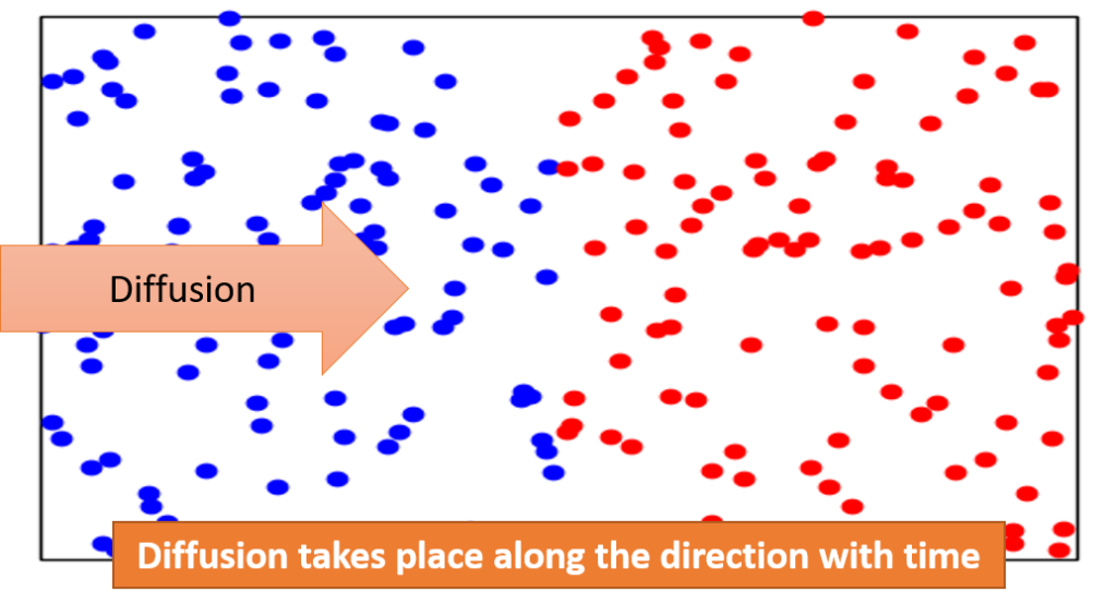
The Fick’s Second Law is important in understanding processes where concentration gradients change over time. For example in Drug Delivery, when a medicated patch is applied on the skin, the drug molecules diffuse from the patch into the bloodstream, therefore how fast this process occurs can be found out with the help of this law.
Mathematically, Fick’s second law of Diffusion equation in one dimension is given by:
\[ \frac{\partial C}{\partial t} = D \frac{\partial^2 C}{\partial x^2} \]
where: –
- \(C\) is the concentration of the solute (a function of position \(x\) and time \(t\)),
- \(t\) is time,
- \(D\) is the diffusion coefficient (assumed to be constant),
- \(x\) is the position
In three dimensions, above equation can be generalized to:
\[ \frac{\partial C}{\partial t} = D \left( \frac{\partial^2 C}{\partial x^2} + \frac{\partial^2 C}{\partial y^2} + \frac{\partial^2 C}{\partial z^2} \right) \]
where \(y\) and \(z\) are the other spatial coordinates.
Related: Fick’s first law of diffusion calculator
Related: Other Mass Transfer Calculators and concepts
Fick’s Second Law of Diffusion Derivation
Let’s consider a one-dimensional system (e.g., a rod or a membrane) where mass is conserved. The equation for mass conservation is:
\( \frac{\partial \phi}{\partial t} + \frac{\partial J}{\partial x} = 0 \)
Rearrange this equation and making flux terms isolate, we get:
\( \frac{\partial \phi}{\partial t} – \frac{\partial}{\partial x} \left(D \frac{\partial \phi}{\partial x}\right) = 0 \)
Now. assuming Constant Diffusion Coefficient (D), and using the equation from fick’s first law of diffusion we get,
\( \frac{\partial}{\partial x} \left(D \frac{\partial \phi}{\partial x}\right) = D \frac{\partial^2 \phi}{\partial x^2} \)
This gives us the form of Fick’s second law:
\( \frac{\partial \phi}{\partial t} = D \frac{\partial^2 \phi}{\partial x^2} \) ——— Eq 1
Equation 1 describes how the concentration \((\phi)\) changes with time due to diffusion i.e Fick’s second law of diffusion. This equation tells us that the rate of change of concentration with respect to time is proportional to the second derivative of concentration with respect to position.
Related: Hydraulic Diameter Calculator for Circular and Non-Circular cross-section
How does temperature affect diffusion according to Fick’s second law?
The diffusion coefficient \((D)\) quantifies how quickly a substance diffuses through a medium. Usually, at higher temperatures, the diffusion coefficient increase because molecules have more thermal motion (kinetic energy) at higher temperatures.
Take Away: The faster the molecules move, the more likely they are to diffuse from regions of high concentration to low concentration.
According the Arrhenius relation, the relationship between the diffusion coefficient and temperature can be expressed using the Arrhenius equation:
\( D = D_0 e^{- \frac{Q_d}{RT}} \)
where:
- \( D_0 \) is the temperature-independent pre-exponential factor
- \( Q_d \) represents the activation energy for diffusion
- \( R \) is the gas constant.
- \( T \) is the absolute temperature (in Kelvin)
As temperature increases, the exponential term \( e^{- \frac{Q_d}{RT}} \) becomes larger, leading to a higher diffusion coefficient.
For example: Imagine a cup of hot coffee. The coffee aroma molecules (substance A) diffuse more rapidly into the air at higher temperatures.
Related: Python code for fick’s first law
Fick’s Second Law for Constant Concentration Source and Diffusion Length
Consider a semi-infinite bar with a constant source (i.e., constant concentration) of solute material diffusing in from one end. with time \(t\) in one dimension (taken as the x-axis) from a boundary located at position \(x = 0\), where the concentration is maintained at a value \(C_0\) as shown in diagram below:
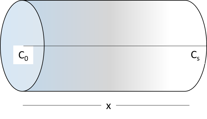
Let’s denote \(C_0\) as the initial concentration of solute in the bar, \(C_s\) as the constant concentration of solute at the end of the bar. The concentration at the end the bar is given as:
\(C(x,t) = C_0 \, \text{erfc} \left( \frac{x}{2\sqrt{Dt}} \right)\)
where \(\text{erfc}\) is the complementary error function, which can be computed using numerical methods or through integral function. The length \(2\sqrt{Dt}\) is called the diffusion length and provides a measure of how far the concentration has propagated in the x-direction by diffusion in time t
For the quick approximation of the error function, the first two terms of the Taylor series can be used, on solving above equation we get:
\(C – C_s = (C_0 – C_s) \cdot erf \left( \frac{x}{2\sqrt{Dt}} \right)\)
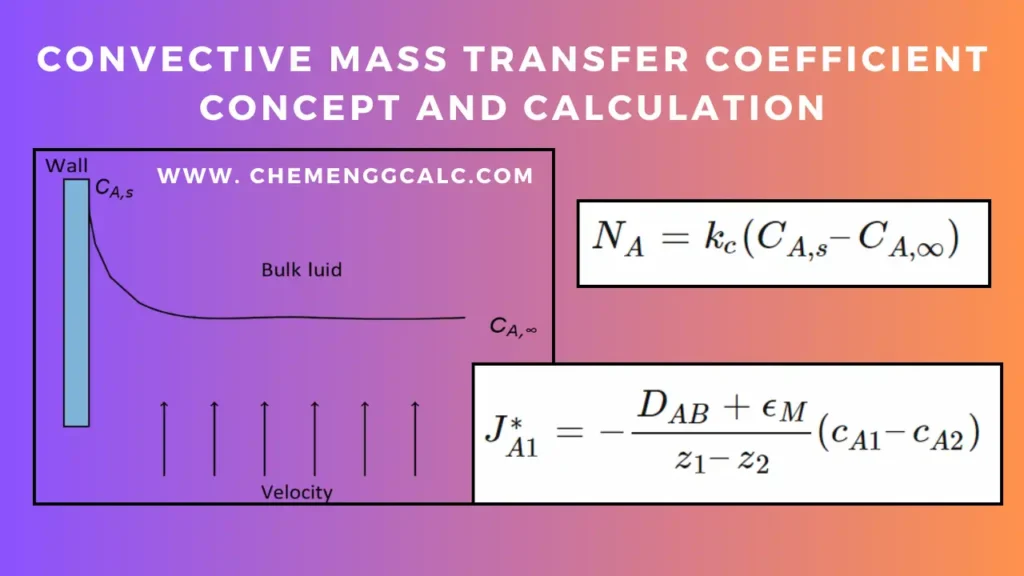
Related: Convective Mass Transfer Coefficient – Concept and Calculation
Example Problem on Fick’s Second Law of Diffusion
An FCC iron-carbon alloy initially containing 0.35 wt % C is exposed to an oxygen-rich and virtually carbon-free atmosphere at 1400 K (1127 \(^{\circ}\)C). Under these circumstances, the carbon diffuses from the alloy and reacts at the surface with the oxygen in the atmosphere, that is, the carbon concentration at the surface position is maintained essentially at 0 wt % C. (This process of carbon depletion is termed as decarburization.) The value of D at 1400 K is \(6.9 \times 10^{-11}\) \(m^2 /s\). At what distance the carbon concentration is 0.15 wt % after a 10-h treatment.
The given problem can be solved with the help of Fick’s Seconds Law of Diffusion:
\( C – C_s = (C_o – C_s) \cdot erf \left( \frac{X}{2\sqrt{Dt}} \right)\)
here:
– \(C\) is the concentration at a depth \(X\) after time \(t\),
– \(C_o\) is the initial concentration,
– \(C_s\) is the surface concentration, and
– \(D\) is the diffusion coefficient.
Given that \(C_s = 0 wt \%\) and \(C_o = 0.35 wt \%\),
It is required to find \(X\) when \(C = 0.15 wt \%\).
Rearranging the equation for \(X\), we get:
\(X = 2\sqrt{Dt} \cdot erfinv \left( \frac{C – C_s}{C_o – C_s} \right)\)
Substituting the given values into the equation:
– \(erfinv(0.15 / 0.35) = 0.3856\)
– \(D = 6.9 \times 10^{-11} m^2/s\)
– \(t = 10\) hours or \(36,000\) seconds
We find that \(X = 1261.4 \mu m\).
Therefore, At a distance of 1.26 mm from the surface, the carbon concentration is 0.15 wt % after a 10-h treatment.
Also Read: Thermal Boundary Layer Thickness (δT) for Flat Plate
Python Code for Fick’s Second Law of Diffusion
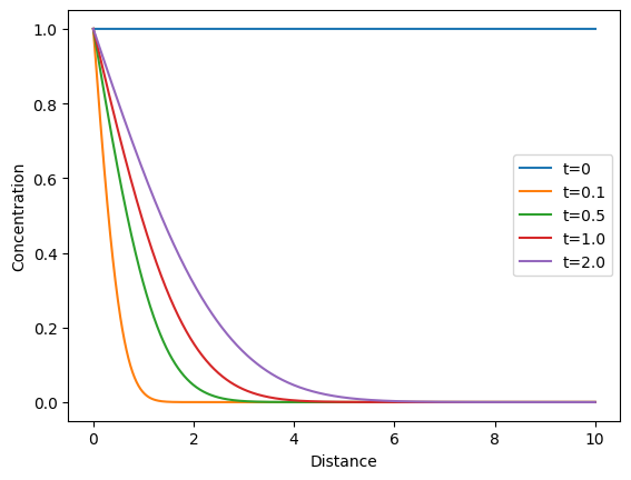
This Python code helps user to calculate and visualizes the concentration profile of a diffusing substance over time and distance, based on Fick’s second law of diffusion. The concentration profiles are calculated at different specified times and plotted against distance.
Note: This Python code solves the specified problem. Users can copy the code and run it in a suitable Python environment. By adjusting the input parameters, users can observe how the output changes accordingly
import numpy as np
import matplotlib.pyplot as plt
from scipy.special import erfc

# Constants
D = 1.0  # Diffusion coefficient
L = 10.0  # Length of the domain
C0 = 1.0  # Initial concentration
times = [0.1, 0.5, 1.0, 2.0]  # Times at which to compute the solution

# Spatial grid
x = np.linspace(0, L, 1000)

# Plot the initial condition
plt.plot(x, np.ones_like(x)*C0, label="t=0")

# Compute the solution at the given times
for t in times:
    C = C0 * erfc(x / (2 * np.sqrt(D * t)))
    plt.plot(x, C, label=f"t={t}")

# Show the plot with a legend
plt.xlabel('Distance')
plt.ylabel('Concentration')
plt.legend()
plt.show()
Output:
Resources
- “Transport Phenomena” by R. Byron Bird, Warren E. Stewart, and Edwin N. Lightfoot.
- “Introduction to Chemical Engineering Thermodynamics” by J.M. Smith, H.C. Van Ness, and M.M. Abbott.
- “Mass Transfer Operations” by Robert E. Treybal.
- Research Papers: Some papers provide Python code snippets for diffusion equations.
- Wikipedia – https://en.wikipedia.org/wiki/Fick%27s_laws_of_diffusion
Disclaimer: The Solver provided here is for educational purposes. While efforts ensure accuracy, results may not always reflect real-world scenarios. Verify results with other sources and consult professionals for critical applications. Contact us for any suggestions or corrections.



My family always say that I am wasting my time here at net, but I
know I am getting know-how every day by reading such nice articles or
reviews.