Fick’s First Law of Diffusion Calculator – Molecular Diffusion

Molecular diffusion is the process by which molecules move from an area of higher concentration to an area of lower concentration, driven by random thermal motion. It is a fundamental mechanism for the transport of substances in gases, liquids, and solids.

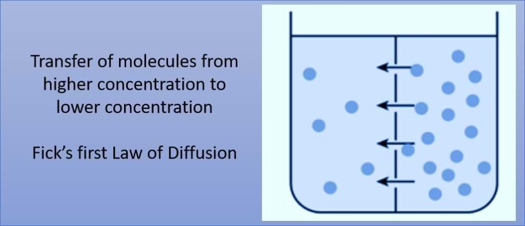
Fick’s first law of diffusion states that the rate of diffusion of a substance across a medium is directly proportional to the concentration gradient of that substance. In simpler terms, it describes how molecules move from an area of high concentration to an area of low concentration over time.

Mathematically Fick’s first law can be expressed as:

\[ J = -D_{AB} \frac{{dC}}{{dx}} \]

where:

• \( J \) represents the flux of the substance (amount of substance passing through a unit area per unit time).
• \( D_{AB} \) is the diffusion coefficient (transfer from solution A to solution B)
• \( \frac{{dC}}{{dx}} \) is the concentration gradient, representing the change in concentration over a distance in x direction.

The negative sign indicates that the flux \(J\) is in the direction of decreasing concentration, which is from the region of higher concentration to the region of lower concentration. In other words, it shows that diffusion occurs down the concentration gradient.

Related: Heat Transfer Calculators

Related: Fick’s second law of Diffusion

Fick’s First Law of Diffusion Calculator

This calculator computes the diffusion rate according to Fick’s Law of Diffusion, allowing users to input parameters such as surface area, initial and final concentrations, distance, and diffusion coefficient.

Significance of Diffusion Coefficient or Diffusivity

The diffusion coefficient is a measure of how quickly particles spread out or diffuse in a particular medium. It quantifies the rate at which particles move from areas of high concentration to areas of low concentration, which is a fundamental process in various natural and synthetic systems, including gases, liquids, and solids.

The diffusion coefficient 𝐷 can be determined experimentally, or through mathematical modelling and simulation based on known physical properties of the system.

The diffusion coefficient can be affected by temperature through an activation energy term. The Arrhenius equation is commonly used to describe this temperature dependence:

\( D = D_0 \exp \left( -\frac{E_a}{RT} \right) \)

where:

• \( D \) is the diffusion coefficient at temperature \( T \),
• \( D_0 \) is the pre-exponential factor or frequency factor,
• \( E_a \) is the activation energy for diffusion,
• \( R \) is the gas constant,
• \( T \) is the absolute temperature in Kelvin.

This equation tells that as temperature increases, the diffusion coefficient also increases exponentially due to the decrease in the activation energy barrier for diffusion. Conversely, at lower temperatures, diffusion slows down due to the higher activation energy required for particles to overcome barriers and move through the medium.

Example Problem on Fick’s First law of Diffusion

A sheet of steel, \(1.5\) mm thick, is exposed to nitrogen atmospheres on both sides at \(1200\) degrees Celsius, reaching a steady-state diffusion condition. The diffusion coefficient for nitrogen in steel at this temperature is \(6 \times 10^{-11} \, \text{m}^2/\text{s}\), and the diffusion flux is measured at \(1.2 \times 10^{-7} \, \text{kg/m}^2\text{s}\). Additionally, the concentration of nitrogen at the high-pressure surface is \(4 \, \text{kg/m}^3\). How far into the sheet, from this high-pressure side, will the concentration be \(2.0 \, \text{kg/m}^3\)? Assume a linear concentration profile.

Given that the diffusion coefficient for nitrogen in steel at 1200 degrees Celsius is \(6 \times 10^{-11} \, \text{m}^2/\text{s}\) and the diffusion flux is \(1.2 \times 10^{-7} \, \text{kg/m}^2\text{s}\),

we apply Fick’s law of diffusion:

\( \text{Flux} = -D \frac{dC}{dx} \)

Where:

Flux = 1.2×10⁻⁷ kg/m²s
D = 6×10⁻¹¹ m²/s

Solving for \(\frac{dC}{dx}\), we find \(\frac{dC}{dx} = -2000\).

Now, integrating this gradient equation:

\( -2000 = \frac{4 \, \text{kg/m}^3 – 2 \, \text{kg/m}^3}{x_B – 0} \)

solving for \(x_B\) to find:

\( x_B = \frac{2}{2000} = 0.001 \, \text{m} \)

Hence, the concentration will reach \(2.0 \, \text{kg/m}^3\) at a distance of \(0.001 \, \text{m}\) from the high-pressure side of the sheet.

Related: 10 Mostly used Dimensionless Numbers in Chemical Engineering

Related: Schmidt Number Calculator – Significance and Calculation

Python Code for Fick’s First Law of Diffusion

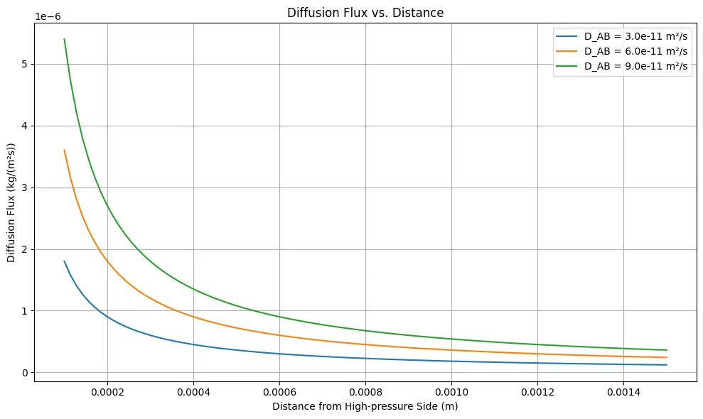
This code computes the diffusion flux across a distance in a material, according to Fick’s first law of diffusion. It takes into account parameters such as the diffusion coefficient and the concentration gradient to determine the rate at which a substance diffuses through the material over a given distance.

Note: This Python code solves the specified problem. Users can copy the code and run it in a suitable Python environment. By adjusting the input parameters, users can observe how the output changes accordingly.

import numpy as np
import matplotlib.pyplot as plt

def calculate_diffusion_flux(D_AB, dC_dx):
    """
    Calculate the diffusion flux using Fick's first law of diffusion.
    
    Parameters:
        D_AB (float): Diffusion coefficient.
        dC_dx (float): Concentration gradient.
    
    Returns:
        float: Diffusion flux.
    """
    flux = -D_AB * dC_dx
    return flux

# Define parameters
initial_concentration = 8  # kg/m³
final_concentration = 2  # kg/m³
x = np.linspace(0.0001, 0.0015, 100)  # Distance from the high-pressure side (m)

# Different values of diffusion coefficients
diffusion_coefficients = [3e-11, 6e-11, 9e-11]  # m²/s

# Plotting
plt.figure(figsize=(10, 6))

for D_AB in diffusion_coefficients:
    # Calculate concentration gradient
    dC_dx = (final_concentration - initial_concentration) / x

    # Calculate diffusion flux
    flux = calculate_diffusion_flux(D_AB, dC_dx)

    # Plot diffusion flux
    plt.plot(x, flux, label=f'D_AB = {D_AB:.1e} m²/s')

plt.title("Diffusion Flux vs. Distance")
plt.xlabel("Distance from High-pressure Side (m)")
plt.ylabel("Diffusion Flux (kg/(m²s))")
plt.grid(True)
plt.legend()
plt.tight_layout()
plt.show()

Output:

Resources:

1. “Transport Phenomena” by R. Byron Bird, Warren E. Stewart, and Edwin N. Lightfoot.
2. “Introduction to Chemical Engineering Thermodynamics” by J.M. Smith, H.C. Van Ness, and M.M. Abbott.
3. “Mass Transfer Operations” by Robert E. Treybal.
4. Research Papers: Some papers provide Python code snippets for diffusion equations.

Disclaimer: The Solver provided here is for educational purposes. While efforts ensure accuracy, results may not always reflect real-world scenarios. Verify results with other sources and consult professionals for critical applications. Contact us for any suggestions or corrections.