Bond Crushing Law and Work Index Calculator (Comminution Laws)

What is Bond Crushing Law ?

Bond Crushing Law or Bond’s Law is one of the more realistic method for estimating the power required for crushing and grinding formulated by F.C. Bond in the 1940s.

Bond’s crushing law states that the work required to form particles of size 𝐷𝑠​ from very large feed is directly proportional to the square root of the surface-to-volume ratio of the product.

Mathematically, Bond’s Law is expressed as:

\[ \frac{P}{\dot{m}} = K_B \cdot \left(\frac{1}{\sqrt{D_{\text{final}}}} – \frac{1}{\sqrt{D_{\text{initial}}}}\right) \]

Where,

• \( P \) is power (in watts or kilowatts),
• \( \dot{m} \) is mass flow rate (in ton/hr),
• \( K_B \) is Bond’s constant, (in \(\text{kW}\cdot\text{h}\cdot\text{m}^{1/2}/\text{ton}\))
• \( D_{\text{final}} \) is the final particle size after crushing (in mm),
• \( D_{\text{initial}} \) is the initial particle size before crushing (in mm).

Note: \(K_B\) is a constant that depends on the type of machine and on the material being crushed, It is calculated experimentally.

Bond’s crushing law is frequently used in the mining and mineral processing industries to evaluate and design crushing and grinding equipment, as well as to optimize the performance of existing equipment.

Related: Sphericity Calculator for different shapes

Work Index

Work Index (𝑊_𝑖​) is a parameter used to quantify the gross energy required in kilowatt hours per ton of feed needed to reduce a very large feed to such a size that 80% of the crushed product is finer than a 100 microns size. It is derived from Bond’s Law, which relates the energy required for comminution (crushing and grinding) to the feed and product particle sizes.

\(K_b\) = 0.3162 * (𝑊_𝑖​)

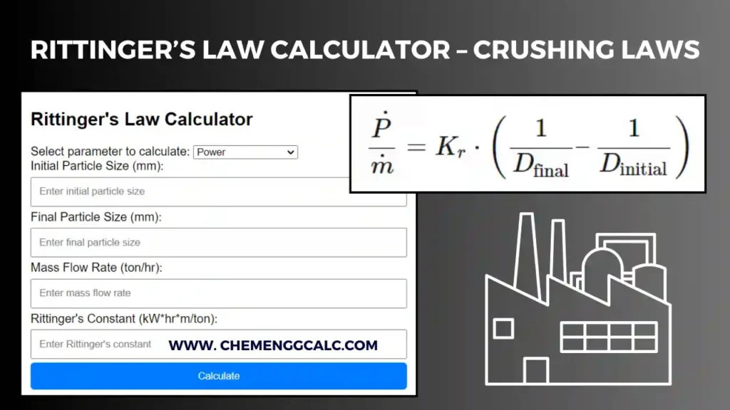
Related: Rittinger’s Law Calculator

Related: Kick’s Law Calculator

Bonds Crushing Law Calculator

The Bond Crushing Law calculator calculates the energy required for crushing of a solid material based on Bond’s Law. It helps in predicting the energy needed to reduce the size of a given material from a specified initial size to a desired final size.

Example Problem on Bonds Crushing Law and Work Index

What is the power required to crush 100 ton/h of limestone if 80 percent of the feed passes a 2-in. screen and 80 percent of the product a -in. screen. work index for limestone is 12.74?

Given:

• Mass flow rate (\(m\)) = 100 ton/h
• Initial particle size (\(D_{\text{feed}}\)) = 2 inches = 50.8 mm
• Final particle size (\(D_s\)) = 1/8 inch = 3.175 mm
• Work Index for limestone (\(W_i\)) = 12.74

Using Bond’s Law formula: \( P = m \cdot K_b \cdot \left(\frac{1}{\sqrt{D_{\text{f}}}} – \frac{1}{\sqrt{D_i}}\right) \)

Substituting the given values: \( P = 100 \times 0.3162 \times \left(\frac{1}{\sqrt{50.8}} – \frac{1}{\sqrt{3.175}}\right) \)

\( P \approx 169.6 \text{ kW} \)

So, the power required to crush 100 ton/h of limestone is approximately 169.6 kW, or approximately 227 hp.

Python Code for Bond Crushing Law

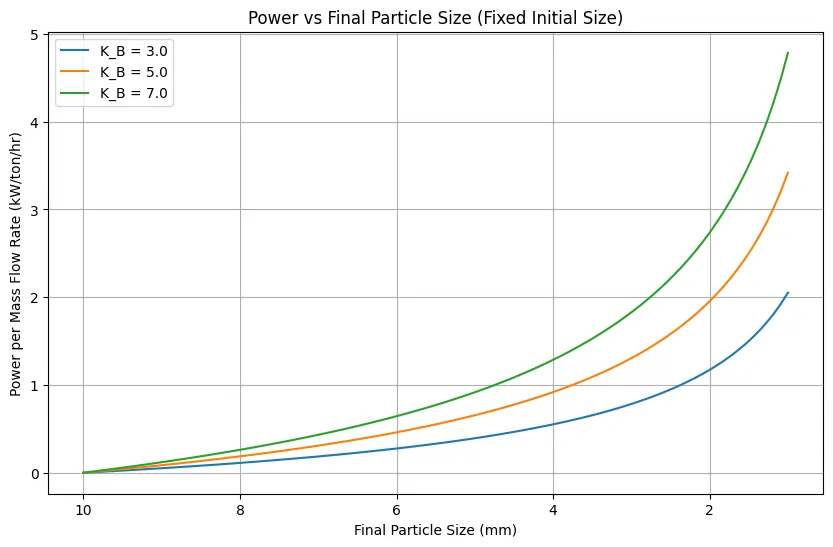
This code calculates the power consumption for size reduction in a crushing process according to Bond’s Law. The initial and final particle sizes of the material being crushed, the mass flow rate of the material, and Bond’s constant are taken then plots the relationship between different values of final size and the corresponding power consumption in kilowatts (kW) for the given process parameters.

Note: This Python code solves the specified problem. Users can copy the code and run it in a suitable Python environment. By adjusting the input parameters, users can observe how the output changes accordingly.

import numpy as np
import matplotlib.pyplot as plt

# Function to calculate power for Bond crushing law
def calculate_power(K_B, D_initial, D_final):
    return K_B * (1/np.sqrt(D_final) - 1/np.sqrt(D_initial))

# Constants
K_B_values = [3.0, 5.0, 7.0]  # Different Bond's constants (kW·h·m^(1/2)/ton)
D_initial = 10.0  # Initial particle size (mm)
D_final = np.linspace(1, 10, 100)  # Final particle size (mm)

# Plotting
plt.figure(figsize=(10, 6))

for K_B in K_B_values:
    # Calculate power
    P_dotm = calculate_power(K_B, D_initial, D_final)
    
    # Plot
    plt.plot(D_final, P_dotm, label=f'K_B = {K_B}')

plt.title('Power vs Final Particle Size (Fixed Initial Size)')
plt.xlabel('Final Particle Size (mm)')
plt.ylabel('Power per Mass Flow Rate (kW/ton/hr)')
plt.grid(True)
plt.gca().invert_xaxis()  # Reverse x-axis
plt.legend()
plt.show()

Output:

Resources:

• “Unit Operations in Chemical Engineering” (McCabe et al.)
• “Particle Technology and Separation Processes” (Richardson et al.)
• “Chemical Engineering Design: Principles, Practice and Economics of Plant and Process Design” (Towler and Sinnott)

Disclaimer: The Solver provided here is for educational purposes. While efforts ensure accuracy, results may not always reflect real-world scenarios. Verify results with other sources and consult professionals for critical applications. Contact us for any suggestions or corrections.