Table of Contents
Residence Time Distribution (RTD) is a very useful concept in chemical engineering that explains distribution of material or fluid element flowing through vessel or reactor such as CSTR and PFR. RTD measurement is important for optimizing reactor performance and ensuring efficient reaction conditions.
Plug Flow and Mixed Flow (CSTR) are the two major flow patterns which leads to different reactor sizes and product distributions. Reactor design are done by approximation of these flow patterns for a given process. However, In real reactors deviations must be considered and here RTD plays its role.
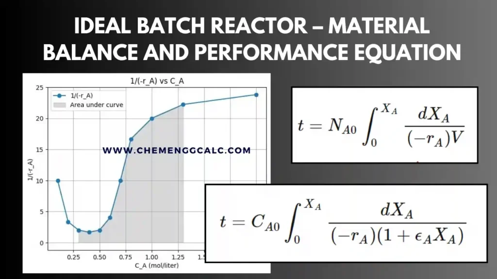
Related: Ideal Batch Reactor – Material Balance and Performance equation Calculations
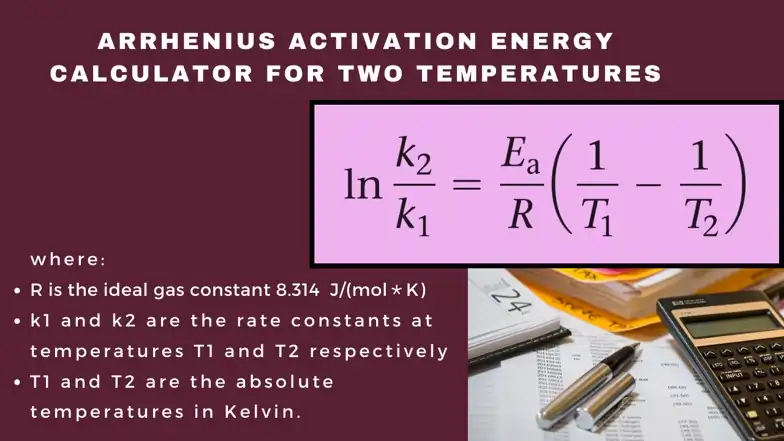
Related: Arrhenius Activation Energy Calculator for two temperatures
Residence Time Distribution Meaning
Residence Time Distribution (RTD) refers to the probability distribution that quantifies how much time fluid elements spend inside a control volume before it exits.
RTD is defined as the probability distribution function E(t), which describes the exit age distribution of fluid particles leaving the reactor after a given time t. E has the unit time-1
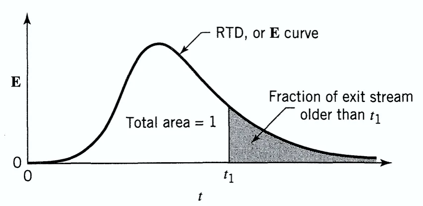
Image Source: Levenspiel, E. J. (1999). Chemical reaction engineering (3rd ed.). Wiley.
The distribution of the exit times, defined as the E(t) curve, is the residence time distribution (RTD) of the fluid. The exit concentration of a tracer species C(t) can be used to define E(t) for an pulse input and the response as follows:
\[E(t) = \frac{C(t)}{\int_0^\infty C(t) \, dt}\]
It is convenient to represent the RTD in such a way that the area under the curve is unity i.e normalizing the distribution for the pulse input and is given as:
\[\int_0^\infty E(t) \, dt = 1 \]
The fraction of the material that leaves the reactor with an time less than t1 is given as::
\[\int_{0}^{t_1} E(t) \, dt\]
The fraction of the material that leaves the reactor with time greater than t1 is given as::
\[\int_{t_1}^\infty E(t) \, dt = 1 – \int_{0}^{t_1} E(t) \, dt\]
The mean residence time is given by the first moment of the age distribution:
\[\bar{t} = \int_{0}^\infty t \cdot E(t) \, dt\]
If there are no dead or stagnant zones within the reactor, then \( \bar{t} \) will be equal to \( \tau \), the residence time calculated from the total reactor volume (V) and the volumetric flow rate (v) of the fluid i.e \(\tau = \frac{V}{v}\)
Related: Plug Flow Reactor – Design Equation and Calculations
Related: C Curve, E Curve and F Curve from Pulse or Step Input Tracer in Non Ideal Reactor
The E curve is the distribution needed to account for non-ideal flow. Higher order central moments provides significant information about the variance and skewness of the E(t) function. Now we will discuss RTD function for CSTR and PFR.

Edition: 3rd Edition, By: Octave Levenspiel
A classic textbook covering the principles of chemical reaction engineering with detailed analysis of reactor design and kinetics.
Buy on AmazonResidence Time Distribution in CSTR (Mixed Flow)
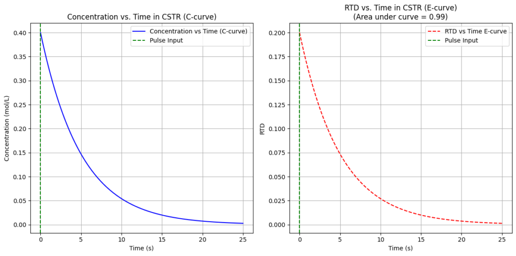
In an ideal CSTR (mixed flow), contents are perfectly mixed which leads to uniform composition throughout the reactor means that every fluid portion has an equal chance of exiting the reactor.
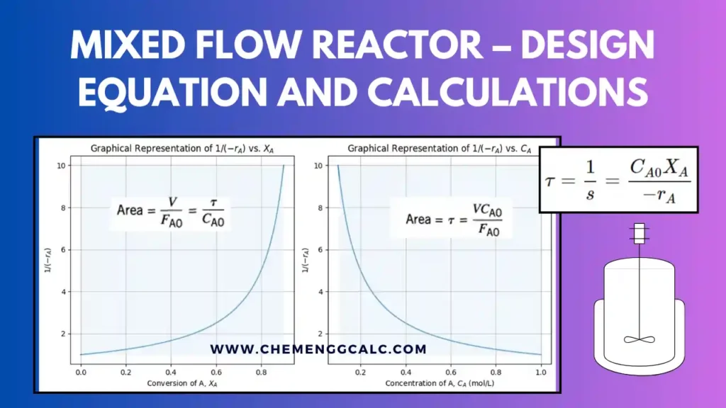
Related: Mixed Flow Reactor – Design Equation and Calculations
The RTD curve for a CSTR is typically an exponential decay function, it shows that some fluid elements exit quickly while others stay longer thus provide the wider distribution of residence times.
The \(E(t)\) function (Exit Age Distribution function) for a CSTR is given by:
\[E(t) = \frac{1}{\tau} e^{-\frac{t}{\tau}}\]
where:
- t is the residence time,
- \( \tau \) is the mean or average residence time.
Characteristics of RTD in CSTR
- Some reactants may leave the reactor before they have had enough time to react.
- The RTD shows a large variance, meaning there is a wide range of residence times.
- No molecule follows the same path, leading to non-uniform performance.
- Multiple peaks suggest issues like channeling, parallel flow paths, or strong internal circulation.
Related: Mixed Flow Reactor – Design Equation and Calculations
Residence Time Distribution in PFR (Plug Flow)
In an ideal Plug Flow Reactor (PFR), there is no mixing in the axial direction, meaning the fluid flows through the reactor uniformly.
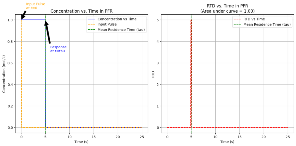
The RTD curve for a PFR is a Dirac delta function, which means that all fluid elements have the same residence time.
The \(E(t)\) function for a PFR is represented as:
\[E(t) = \delta(t – \tau)\]
where, \( \delta(t – \tau) \) is the Dirac delta function centered at the mean residence time \( \tau \).
This equations explains that all fluid elements exit the reactor after spending exactly the same amount of time inside, which equals \( \tau \), the average residence time.
Characteristics of RTD in PFR
- The RTD is narrow, represented by a sharp peak at \( t = \tau \), The variance of an ideal plug-flow reactor is zero.
- Real reactors have RTD curves that differ from ideal reactors due to fluid flow conditions.
- A non-zero variance means there is some dispersion in the fluid, caused by turbulence, uneven velocity, or diffusion.
- If the mean of the RTD curve appears earlier than expected, it may indicate stagnant fluid in the reactor.
- More than one peak in the RTD curve could mean channeling, parallel flow paths, or strong internal circulation.
The RTD provides an important information for designing and optimizing reactors because it directly impacts conversion, selectivity, and overall reactor efficiency.
Related: Conversion, Selectivity, Yield for a multiple reaction
Related: Rate Constant Calculation for Zeroth, First and Second Order using Integrated Rate Equations
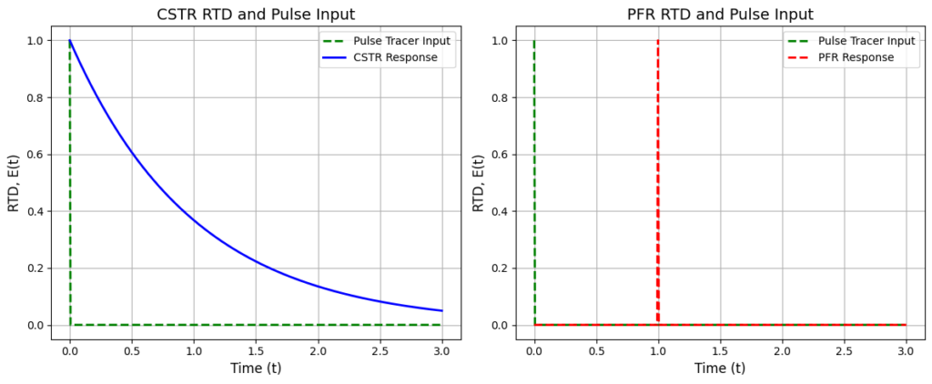
Python Code for RTD in CSTR and PFR
This Python code helps user to visualize and compare the Residence Time Distribution (RTD) for CSTR and PFR. The RTD for the CSTR is modeled as an exponential decay function, while the RTD for the PFR is approximated using a Dirac delta function for a pulse tracer input.
Note: This Python code solves the specified problem. Users can copy the code and run it in a suitable Python environment. By adjusting the input parameters, and observe how the output changes accordingly.
import numpy as np
import matplotlib.pyplot as plt

# Define the mean residence time for both reactors
tau = 1  # Mean residence time

# Time array for plotting (0 to 3*tau)
t = np.linspace(0, 3 * tau, 500)

# RTD for CSTR: E(t) = (1/tau) * exp(-t/tau)
def rtd_cstr(t, tau):
    return (1 / tau) * np.exp(-t / tau)

# RTD for PFR: E(t) = delta(t - tau) is approximated using a sharp peak
def rtd_pfr(t, tau):
    E = np.zeros_like(t)
    E[np.argmin(np.abs(t - tau))] = 1  # Dirac delta approximation
    return E

# Define the pulse tracer input (a sharp peak at t=0)
def pulse_tracer(t):
    pulse = np.zeros_like(t)
    pulse[0] = 1  # Sharp input at t=0
    return pulse

# Create subplots side by side
fig, (ax1, ax2) = plt.subplots(1, 2, figsize=(12, 5))

# Plot CSTR tracer response
ax1.plot(t, pulse_tracer(t), label="Pulse Tracer Input", color="green", lw=2, linestyle='--')
ax1.plot(t, rtd_cstr(t, tau), label="CSTR Response", color="blue", lw=2)
ax1.set_xlabel("Time (t)", fontsize=12)
ax1.set_ylabel("RTD, E(t)", fontsize=12)
ax1.set_title("CSTR RTD and Pulse Input", fontsize=14)
ax1.legend(loc="best")
ax1.grid(True)

# Plot PFR tracer response
ax2.plot(t, pulse_tracer(t), label="Pulse Tracer Input", color="green", lw=2, linestyle='--')
ax2.plot(t, rtd_pfr(t, tau), label="PFR Response", color="red", lw=2, linestyle='--')
ax2.set_xlabel("Time (t)", fontsize=12)
ax2.set_ylabel("RTD, E(t)", fontsize=12)
ax2.set_title("PFR RTD and Pulse Input", fontsize=14)
ax2.legend(loc="best")
ax2.grid(True)

# Adjust layout and display the plot
plt.tight_layout()
plt.show()
Output:
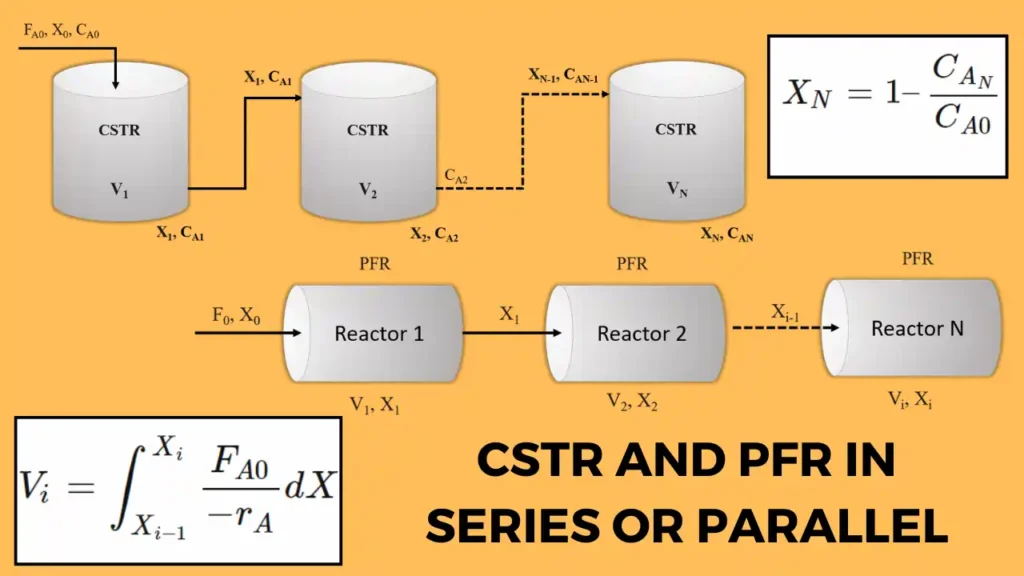
Related: PFR and CSTR in Series or Parallel Combination for a single reaction
Example Problem to plot RTD Curve
In an Experiment, The concentration readings (shown in table below) represent a continuous response to a pulse input into a closed vessel which is to be used as a chemical reactor. Calculate the mean residence time of fluid in the vessel t, and tabulate and plot the exit age distribution E?
| Time (t, min) | Tracer Output Concentration (Cpulse, gm/liter) |
|---|---|
| 0 | 0 |
| 5 | 3 |
| 10 | 5 |
| 15 | 5 |
| 20 | 4 |
| 25 | 2 |
| 30 | 1 |
| 35 | 0 |
Solution:
Let’s first calculate the mean residence time \(\tau\) using formula:
\[ \tau = \frac{\sum(t \cdot C \cdot \Delta t)}{\sum(C \cdot \Delta t)} \]
where:
- t is the time given
- C is the concentration at given time t
- \(\Delta t\) is the time interval between measurements
| Time t, min | Tracer Output Concentration | Δt | t * C | C * Δt | t * C * Δt |
|---|---|---|---|---|---|
| 0 | 0 | 5 | 0 | 0 | 0 |
| 5 | 3 | 5 | 15 | 15 | 75 |
| 10 | 5 | 5 | 50 | 25 | 250 |
| 15 | 5 | 5 | 75 | 25 | 375 |
| 20 | 4 | 5 | 80 | 20 | 400 |
| 25 | 2 | 5 | 50 | 10 | 250 |
| 30 | 1 | 5 | 30 | 5 | 150 |
| 35 | 0 | 5 | 0 | 0 | 0 |
| 100 | 1500 |
therefore, \( \tau = \frac{1500}{100} = 15 \) min.
Now, the Area covered in the concentration-time cover is:
\[\text{Area} = \sum C \Delta{t}\]
Area = (3+5+5+5+4+2+1)*5 = 100 gm. min./liter
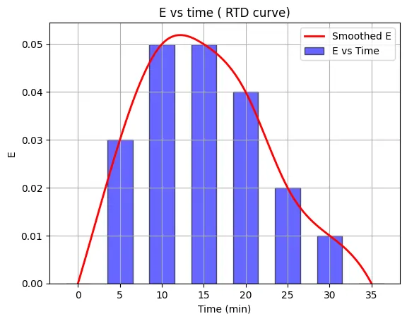
To find the E curve or RTD plot, \( E = \frac {C} {\text{Area}}\)
| Time t, min | Tracer Output Concentration | Area | E = C / Sum of Area |
|---|---|---|---|
| 0 | 0 | 0 | 0 |
| 5 | 3 | 15 | 0.03 |
| 10 | 5 | 25 | 0.05 |
| 15 | 5 | 25 | 0.05 |
| 20 | 4 | 20 | 0.04 |
| 25 | 2 | 10 | 0.02 |
| 30 | 1 | 5 | 0.01 |
| 35 | 0 | 0 | 0 |
| | | 100 | 1 |
The RTD plot is shown below i.e E vs Time plot.
Related: Rate Constant Calculation for Zeroth, First and Second Order using Integrated Rate Equations
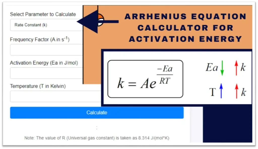
Related: Arrhenius Equation Calculator for Activation Energy
Resources:
- Chemical Reactor Analysis and Design Fundamentals by Rawlings and Ekerdt
- Elements of Chemical Reaction Engineering by Fogler
- “Chemical Reaction Engineering“ by Octave Levenspiel
Disclaimer: The content provided here is for educational purposes. While efforts ensure accuracy, results may not always reflect real-world scenarios. Verify results with other sources and consult professionals for critical applications. Contact us for any suggestions or corrections.