Table of Contents
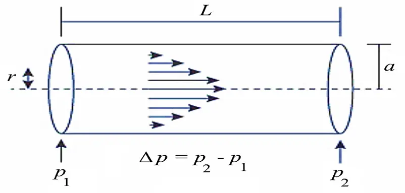
The Hagen-Poiseuille equation, also known as Poiseuille’s Law, is a mathematical equation that describes the flow of an incompressible, Newtonian fluid (a fluid with constant viscosity) through a long cylindrical pipe of constant cross-section.
This law is used primarily in fluid dynamics to predict the volume flow rate of the fluid.

The Hagen-Poiseuille equation is given by:
Q = (π * r^4 * ΔP) / (8 * η * L)
where:
- Q is the Volumetric flow rate (in cubic meters per second, m3/s)
- r is the Pipe radius (in meters, m)
- ΔP is the Pressure difference across the length of the pipe (in pascals, Pa)
- η is the Dynamic viscosity of the fluid (in pascals-seconds, Pa·s)
- L is the Pipe length (in meters, m)
The equation helps us understand how fluid flows through pipes. It’s applicable to scenarios like air flow in lung alveoli, liquid flow through a drinking straw, or fluid delivery via a hypodermic needle.
Related: Newton’s Law of Viscosity Calculator – Dynamic Viscosity
Related: Other Fluid Mechanics Calculator
Hagen-Poiseuille Equation Calculator
This Hagen-Poiseuille Solver helps user to calculate the Hagen-Poiseuille equation for laminar flow in cylindrical pipes. The user selects a parameter to calculate (e.g., flow rate, radius, pressure difference, viscosity, or pipe length) and inputs the required values.
Related: Reynolds Number Calculator for a Circular Pipe
Related: Newton’s Law of Viscosity Calculator – Dynamic Viscosity
Click here – ASME B31. Piping Package to purchase comprehensive collection of codes for power, fuel gas and process piping. It also includes codes for pipeline transportation, gas transmission and distribution piping, and hydrogen piping. ASME B31. Piping Package includes 10 standards with a 15% discount provided by American Society of Mechanical Engineers [ASME].
Assumptions and limitations for Poiseuille’s Law
- The fluid must be incompressible and Newtonian.
- The flow must be laminar (smooth) through a pipe that is substantially longer than its diameter.
- There should be no acceleration of fluid within the pipe.
- For velocities and pipe diameters above a threshold, actual fluid flow becomes turbulent, leading to larger pressure drops than predicted by the Hagen–Poiseuille equation.
Edition: Revised 2nd Edition, By: R. Byron Bird, Warren E. Stewart, Edwin N. Lightfoot
Comprehensive coverage of transport phenomena, including momentum, heat, and mass transfer. Updated content for better clarity.
Buy on AmazonExample Problem on Poiseuille’s Law
A crude oil of viscosity 0.97 poise and relative density 0.9 is flowing through a horizontal circular pipe of diameter 100 mm and of length 10 m. Calculate the difference of pressure at the two ends of the pipe. If 100kg of oil is collected in a tank in 30 second?
Given data:
- Viscosity (μ): 0.97 poise (0.097 Ns/m2)
- Relative density: 0.9
- Density (ρo): 900 kg/m3
- Diameter of pipe (D): 100 mm (0.1 m)
- Length of pipe (L): 10 m
- Mass of oil (m): 100 kg
- Time (t): 30 seconds
To find: Difference in pressure (P1 – P2)
Formula for pressure difference (for viscous flow): P1 – P2 = 32 * μ * Ū * L / D^2
Average velocity (Ū) = Q / Area
- Mass flow rate (Q) = 100 kg / 30 seconds = 0.0037 m^3/s
- Ū = 0.471 m/s
Reynolds number (Re) = ρ * V * D / μ
- Re = 436.91 (laminar flow)
Using the formula for pressure difference:
P1 – P2 = 32 * μ * Ū * L / D^2 = 32 * 0.097 * 0.471 * 10 / (0.1)2
= 1462.28 N/m2 = 0.1462 N/cm2
Python Code for Solving Hagen-Poiseuille Equation
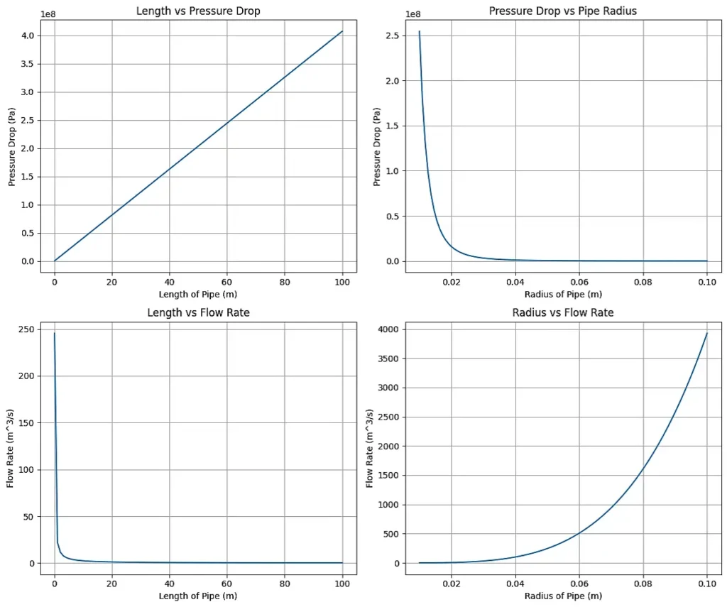
This Python code calculates the volumetric flow rate and pressure drop in a pipe using the Hagen-Poiseuille equation. The input parameters include pipe length, radius, pressure difference, and dynamic viscosity of the fluid. The code then generates a plot which shows the relationship between pipe length and pressure drop, this tool is valuable for analyzing fluid flow systems and designing efficient piping networks.
Note: This Python code solves the specified problem. Users can copy the code and run it in a suitable Python environment. By adjusting the input parameters, users can observe how the output changes accordingly.
"""
Question Statement:

Investigate the relationship between pressure drop, flow rate, and pipe parameters in a fluid flow system using Python.

Given parameters:
- Viscosity: 0.97 poise (0.097 Ns/m^2)
- Relative density: 0.9
- Density: 900 kg/m^3
- Pipe diameter: 100 mm (0.1 m)
- Pipe length: Varies from 0.1 m to 100 m
- Pressure difference: 10,000 Pa

Utilize the Hagen-Poiseuille equation to calculate pressure drop.
Analyze the plots to understand the effects of pipe length and radius on pressure drop and flow rate.

"""

import numpy as np
import matplotlib.pyplot as plt

# Function to calculate pressure drop using Hagen-Poiseuille equation
def hagen_poiseuille(r, delta_P, eta, L):
    return (8 * eta * L * delta_P) / (np.pi * r**4)

# Define parameters
r = 0.05  # Radius of the pipe in meters
delta_P = 10000  # Pressure difference in pascals
eta = 0.001  # Dynamic viscosity of the fluid in pascal-seconds
L = np.linspace(0.1, 100, 100)  # Varying lengths of the pipe in meters
radii = np.linspace(0.01, 0.1, 100)  # Varying radii of the pipe in meters

# Calculate pressure drops corresponding to different lengths
pressure_diff_length = [hagen_poiseuille(r, delta_P, eta, length) for length in L]

# Calculate pressure drops corresponding to different radii
pressure_diff_radius = [hagen_poiseuille(radius, delta_P, eta, L[0]) for radius in radii]

# Calculate flow rates corresponding to different lengths
flow_rate_length = [(np.pi * r**4 * delta_P) / (8 * eta * length) for length in L]

# Calculate flow rates corresponding to different radii
flow_rate_radius = [(np.pi * radius**4 * delta_P) / (8 * eta * L[0]) for radius in radii]

# Create a figure with four subplots
fig, ((ax1, ax2), (ax3, ax4)) = plt.subplots(2, 2, figsize=(12, 10))

# Plot 1: Length vs Pressure Drop
ax1.plot(L, pressure_diff_length)
ax1.set_xlabel('Length of Pipe (m)')
ax1.set_ylabel('Pressure Drop (Pa)')
ax1.set_title('Length vs Pressure Drop')
ax1.grid(True)

# Plot 2: Pressure Drop vs Pipe Radius
ax2.plot(radii, pressure_diff_radius)
ax2.set_xlabel('Radius of Pipe (m)')
ax2.set_ylabel('Pressure Drop (Pa)')
ax2.set_title('Pressure Drop vs Pipe Radius')
ax2.grid(True)

# Plot 3: Length vs Flow Rate
ax3.plot(L, flow_rate_length)
ax3.set_xlabel('Length of Pipe (m)')
ax3.set_ylabel('Flow Rate (m^3/s)')
ax3.set_title('Length vs Flow Rate')
ax3.grid(True)

# Plot 4: Radius vs Flow Rate
ax4.plot(radii, flow_rate_radius)
ax4.set_xlabel('Radius of Pipe (m)')
ax4.set_ylabel('Flow Rate (m^3/s)')
ax4.set_title('Radius vs Flow Rate')
ax4.grid(True)

# Adjust layout
plt.tight_layout()

# Show plot
plt.show()
Output:

Resources:
- “Fluid Mechanics” by Frank M. White
- “Introduction to Fluid Mechanics” by Robert W. Fox, Alan T. McDonald, and Philip J. Pritchard
- “Principles of Heat and Mass Transfer” by Frank P. Incropera and David P. DeWitt
- Python.org – The official Python website offers tutorials, documentation, and resources for learning Python.
Disclaimer: The Solver provided here is for educational purposes. While efforts ensure accuracy, results may not always reflect real-world scenarios. Verify results with other sources and consult professionals for critical applications. Contact us for any suggestions or corrections.
Disclaimer: The Solver provided here is for educational purposes. While efforts ensure accuracy, results may not always reflect real-world scenarios. Verify results with other sources and consult professionals for critical applications. Contact us for any suggestions or corrections.


Could you add a calculator for non-Newtonian fluid flow in microchannels?
yes, surely we will update such calculator, what is your need exactly, what do you want to calculate?